
How do I make the first row in excel a header
 By
SpreadCheaters
By
SpreadCheaters
Microsoft Excel offers a very interesting way to freeze rows. This functionality can be used to make the first row in excel a header. We can perform the below mentioned way to make the first row a header in excel:
We’ll learn about this methodology step by step.
Make the first row a header in excel:
Step-1: Workbook with some data
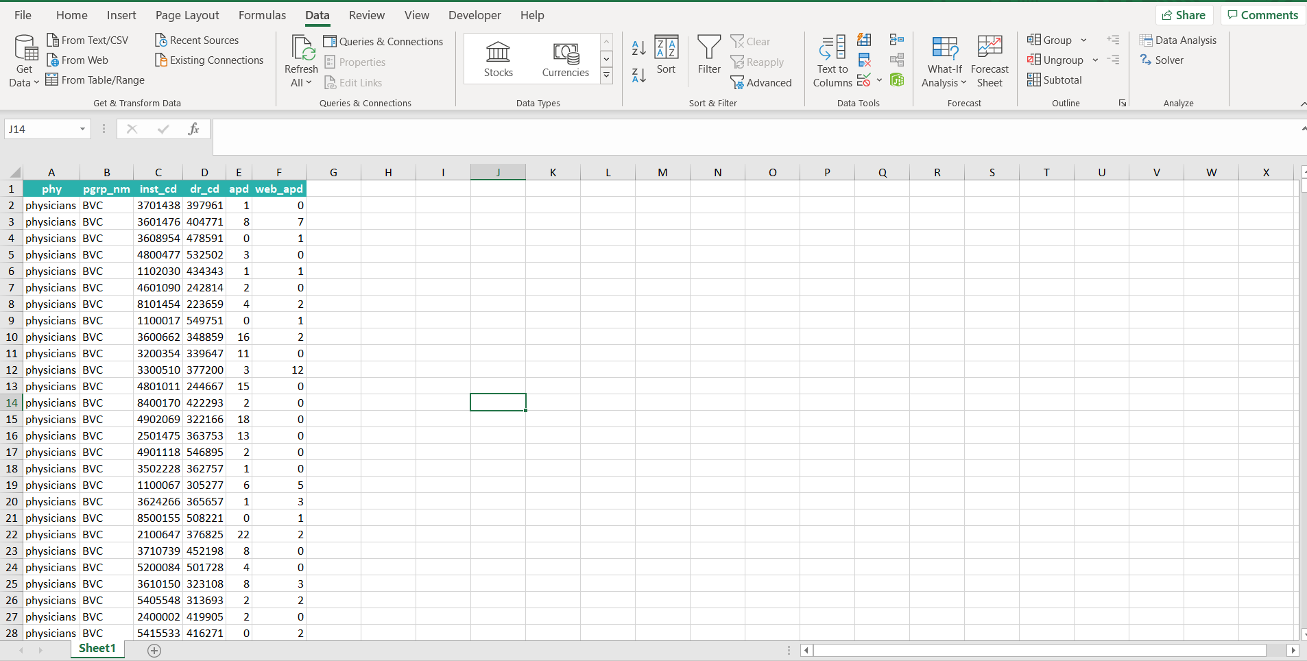
To do this yourself, please follow the steps described below;
– Open the desired Excel workbook in which you want to make the first row a header.
– Now go to the row which is just below the row which you want to make a header. In our case let us go to the second row, and make any cell in this row active, by clicking on any cell in this row.
Step-2: Going to the row below the selected row
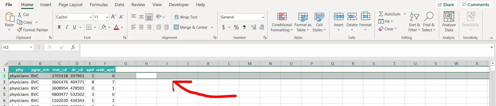
– Now press SHIFT + SPACEBAR in order to select this entire row. In our case, the entire second row should get selected.
Step-3: Selecting the entire row
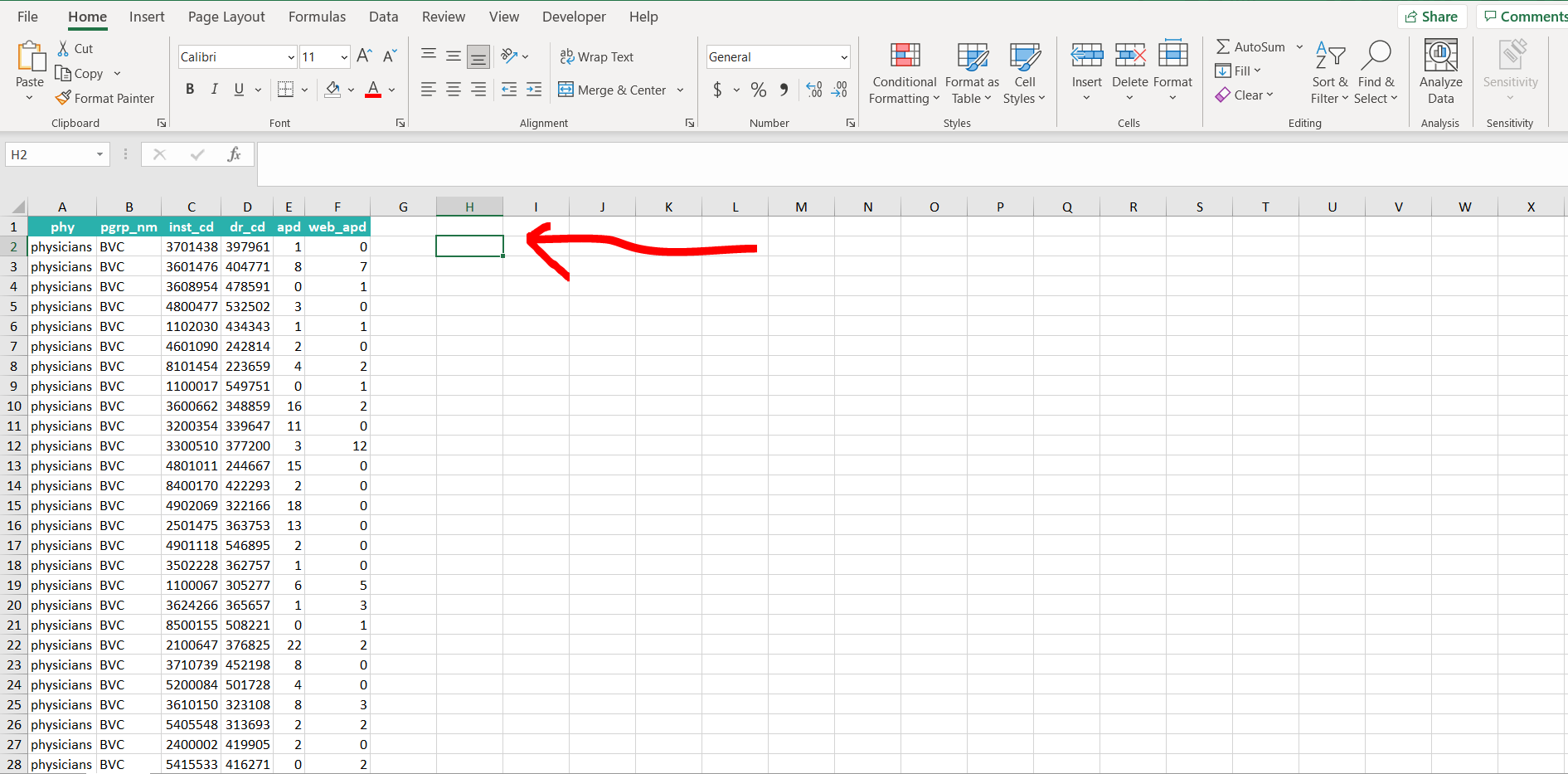
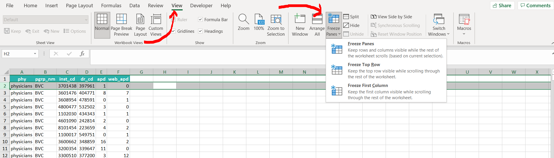
– Now click on the “View” option on the menu bar, and then click on the “Freeze Panes” option. A drop-down menu would appear, as shown in the image below.
Step-4: Navigating through View option in the menu bar
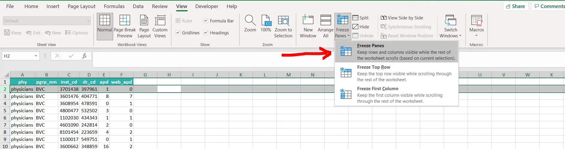
– Now select the “Freeze Panes” option.
Step-5: Selecting the Freeze Panes option
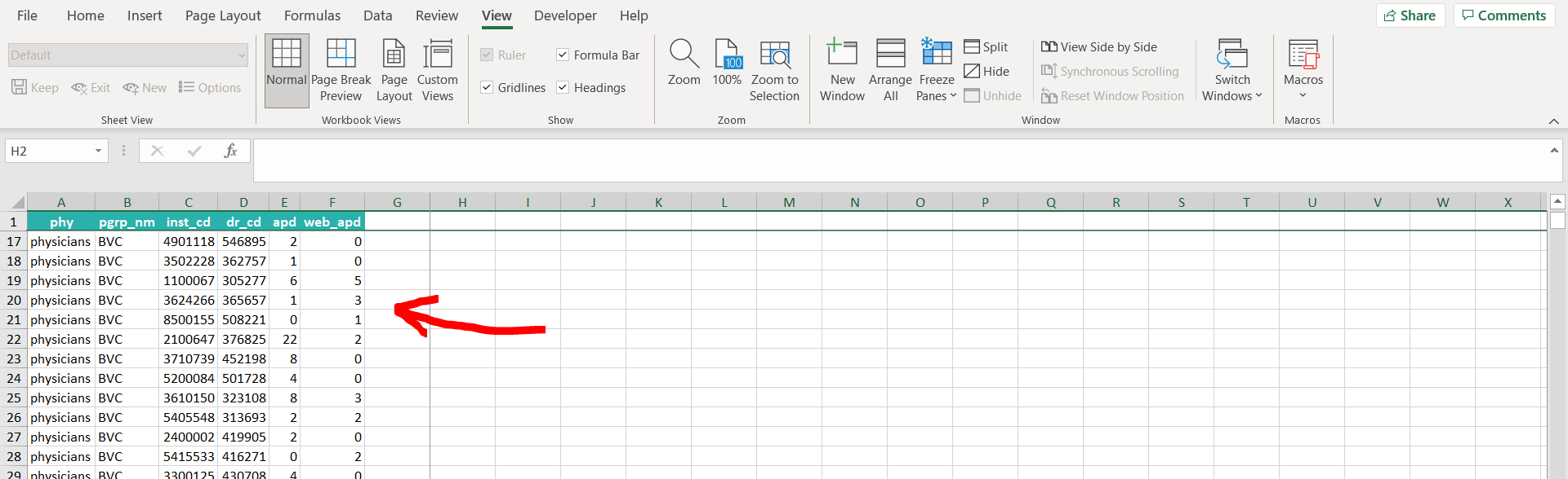
– Now if we try to scroll towards the bottom of the page, we will notice that Row-1 has been frozen. In the image below we can see that after scrolling down the page, Row-1 is still stationary, but the rest of the rows are being scrolled
Final Image: First row has been made the header by freezing
– Additionally, if we want to skip going to the view option, clicking on Freeze panes, and then selecting the freeze panes option, we can use the excel shortcut after selecting the entire row, which is ALT + W + F + F. This will cater to the exact same subject, as we did above.


