
How do I compare two Excel spreadsheets
 By
SpreadCheaters
By
SpreadCheaters
You can watch a video tutorial here.
Comparing two Excel sheets is an operation you will frequently need to do when working with datasets. This happens especially when you are consolidating data from multiple sources. You could compare the sheets by arranging them side-by-side but this method is highly prone to error. Excel provides ways in which this comparison can be automated. The method that you use depends on the type of comparison that you need to do.
In this example, we will look at two scenarios.
- Compare the sheets for missing and matching data. We will compare two lists of customers received from two sales executives and identify the values that are present in both sheets and those that are not. This can be done using the VLOOKUP() function.
- VLOOKUP() function: this searches for a value from Table 1 in the left-most column of a range from Table 2, and returns the value in the column specified from the row of the match in the range of Table 2.
- Syntax: VLOOKUP(lookup_value, table_array, col_index_num, range_lookup)
- lookup_value: the cell reference of the first value in the key column from Table 1
- table_array: the range of Table 2 which is made constant with the addition of dollar signs ($)
- col_index_num: the number of the column in Table 2 that has to be retrieved
- range_lookup: TRUE will return an approximate match, FALSE will return an exact match
- Syntax: VLOOKUP(lookup_value, table_array, col_index_num, range_lookup)
- VLOOKUP() function: this searches for a value from Table 1 in the left-most column of a range from Table 2, and returns the value in the column specified from the row of the match in the range of Table 2.
- Compare the sheets for incorrect and correct data. We will compare two identical lists of customers and identify the order values that match and those that do not. This can be done using the IF() function.
- IF(): this evaluates a condition and returns a value depending on whether the condition is true or false
- Syntax: IF(condition, true, false)
- condition: the condition or statement to be evaluated
- true: the value to be returned if the condition is true
- false: the value to be returned if the condition is false
- Syntax: IF(condition, true, false)
- IF(): this evaluates a condition and returns a value depending on whether the condition is true or false
Option 1 – Compare for missing data
Step 1 – Create a column for missing values on the first sheet
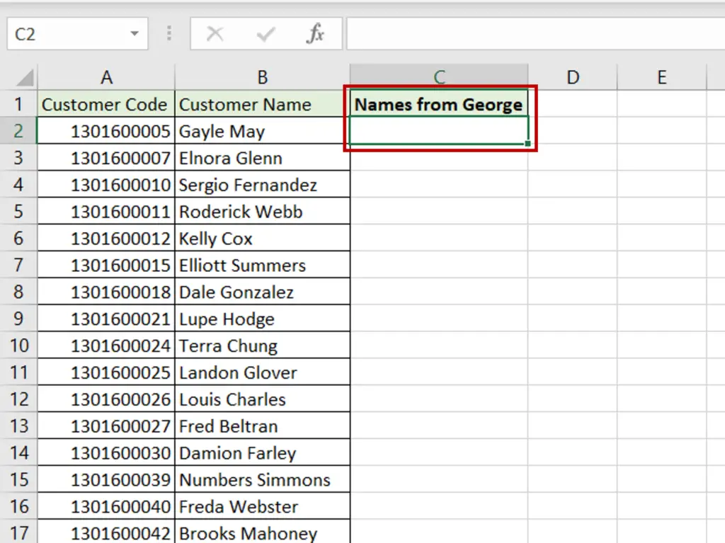
- On the first sheet i.e. ‘Mary’, create a column called ‘Names from George’
- Select the first cell in the column
Step 2 – Create the formula
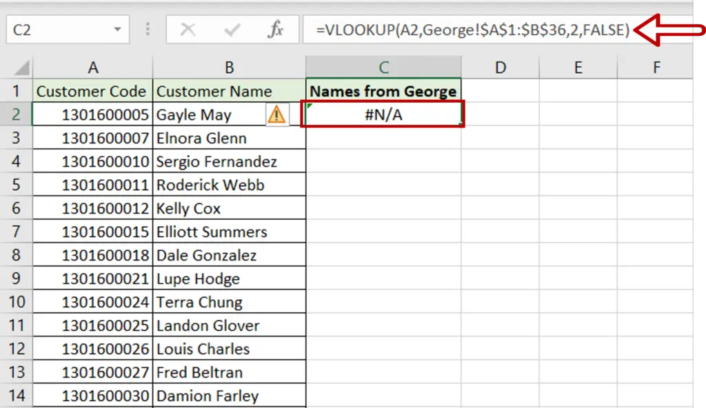
- Type the formula using cell references:
=VLOOKUP(Customer code from ‘Mary’, $Table from ‘George’&,2,FALSE)
- Customer code from ‘Mary’ is the Lookup value
- Table from ‘George’ is the Table-array, made constant by the addition of dollar signs
- 2 is the Col_index_num as the value in the second column is to be returned
- FALSE is the Range_lookup as we need an exact match
- Press Enter
Note: A few things to keep in mind when using Vlookup:
- The key that is common between the tables must always be in the left-most column of Table 2
- Table 2, or the table that is being referred to must always be sorted on the key
- It is better Table 2 has unique values or else this function may not return the desired result
Step 3 – Copy the formula
- Using the fill handle from the first cell, drag the formula to the remaining cells
OR
- Select the cell with the formula and press Ctrl+C or choose Copy from the context menu (right-click)
- Select the rest of the cells in the column and press Ctrl+V or choose Paste from the context menu (right-click)
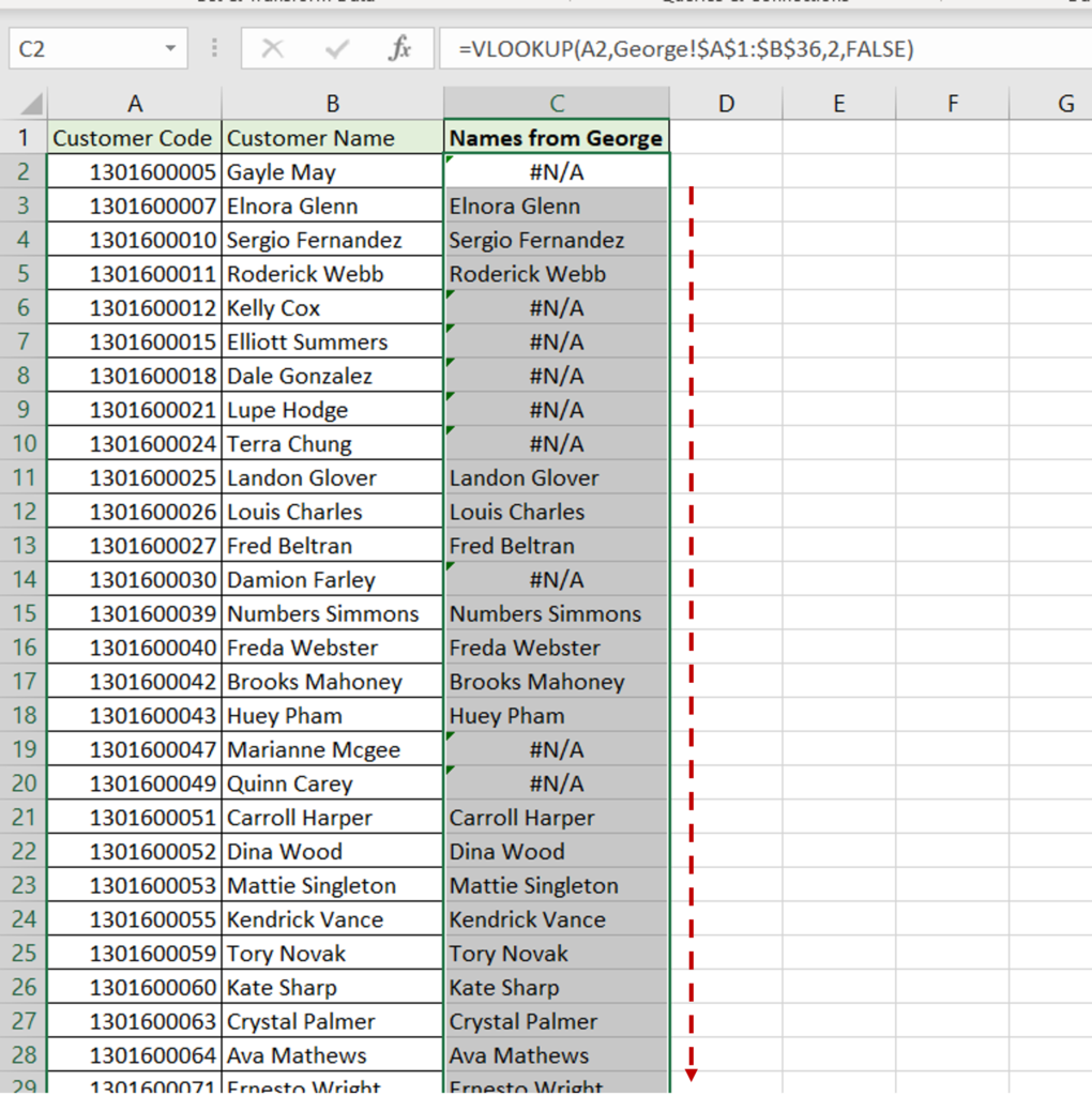
Step 4 – Compare the values
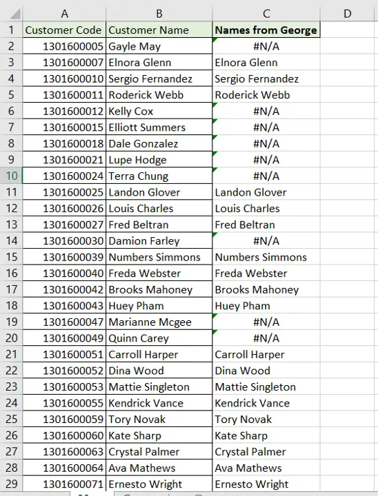
- The customers that are present in the ‘Mary’ sheet and not in the ‘George’ sheet are indicated by the error values i.e. #N/A
- The names are displayed for those customers on both sheets
Step 5 – Create a column for missing values on the second sheet
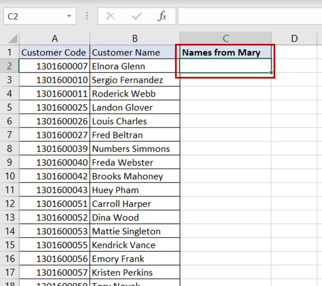
- On the second sheet i.e. ‘George, create a column called ‘Names from Mary’
- Select the first cell in the column
Step 6 – Create the formula
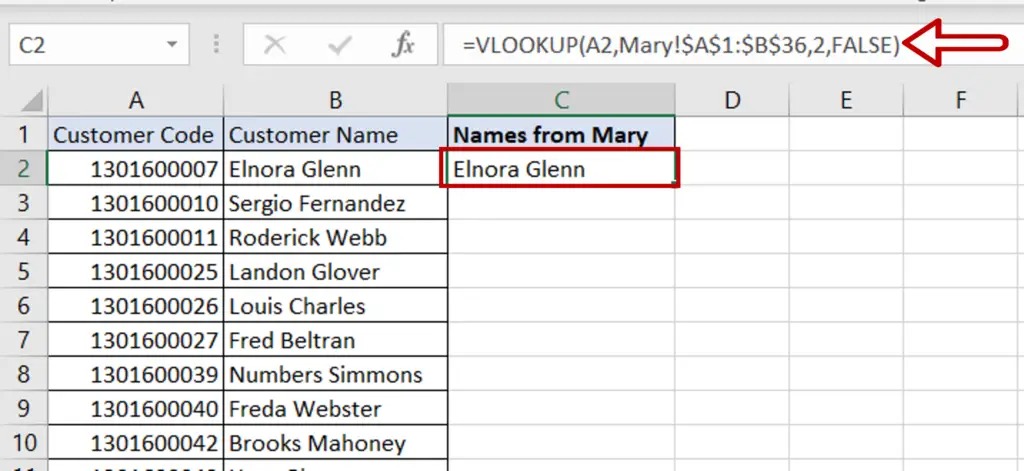
- Type the formula using cell references:
=VLOOKUP(Customer code from ‘George’, $Table from ‘Mary’&,2,FALSE)
- Customer code from ‘George’ is the Lookup value
- Table from ‘Mary’ is the Table-array, made constant by the addition of dollar signs
- 2 is the Col_index_num as the value in the second column is to be returned
- FALSE is the Range_lookup as we need an exact match
- Press Enter
Step 7 – Copy the formula
- Using the fill handle from the first cell, drag the formula to the remaining cells
OR
- Select the cell with the formula and press Ctrl+C or choose Copy from the context menu (right-click)
- Select the rest of the cells in the column and press Ctrl+V or choose Paste from the context menu (right-click)
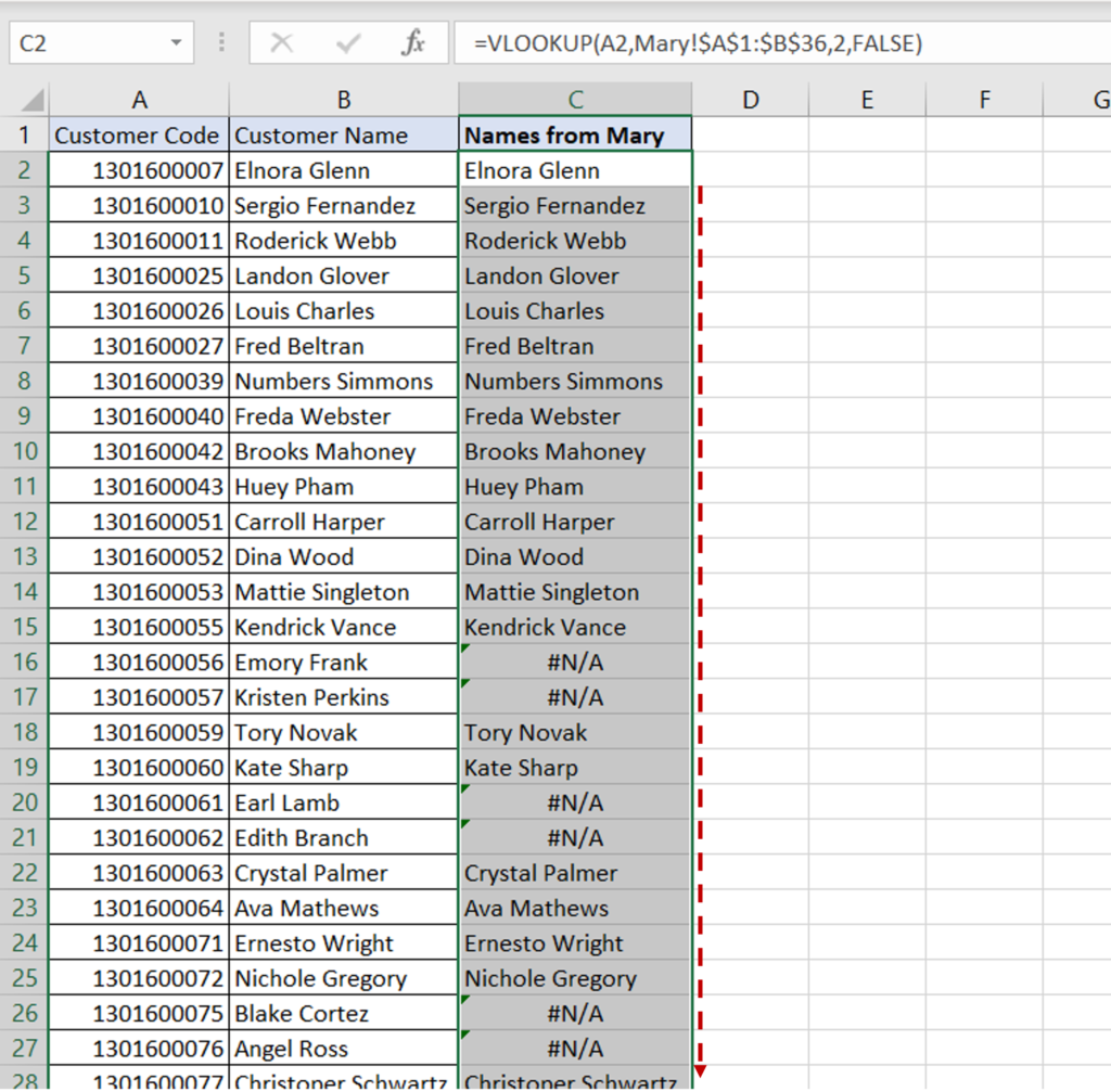
Step 8 – Compare the values
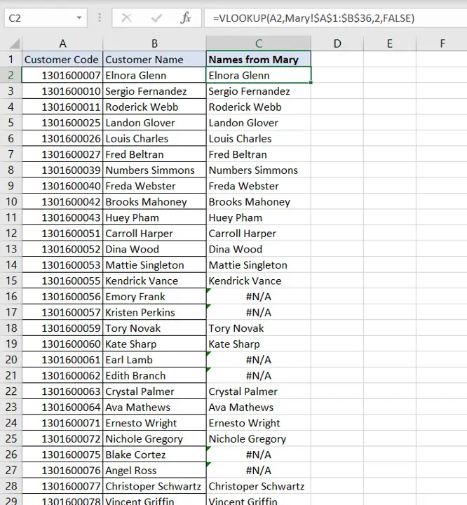
- The customers that are present in the ‘George’ sheet and not in the ‘Mary’ sheet are indicated by the error values i.e. #N/A
- The names are displayed for those customers on both sheets
Option 2 – Compare for incorrect data
Step 1 – Create a column for comparison on the first sheet
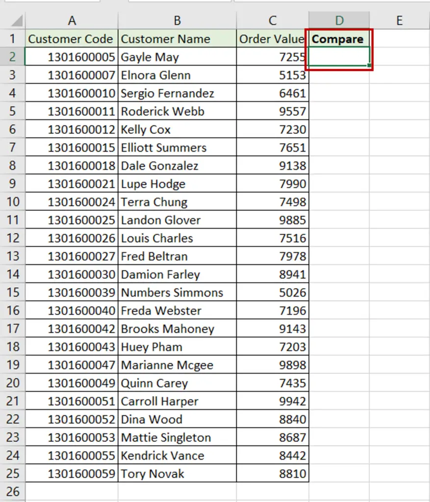
- On the first sheet i.e. ‘21Jan’, create a column called ‘Compare’
- Select the first cell in the column
Step 2 – Create the formula
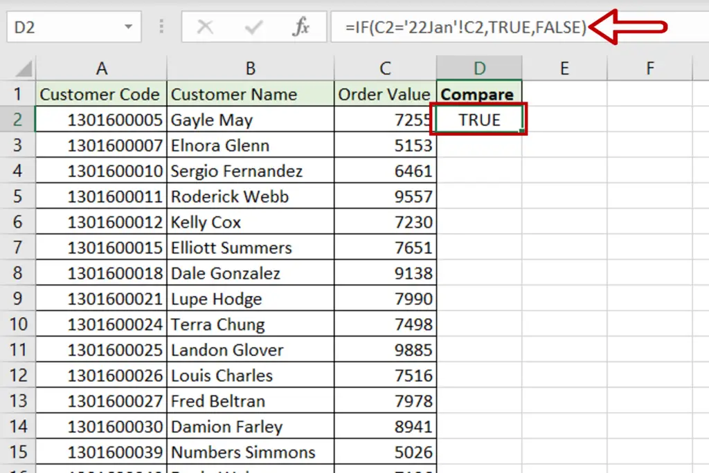
- Type the formula using cell references:
=IF(Order Value from 21Jan = Order Value from 22Jan, TRUE,FALSE)
- Press Enter
Step 3 – Copy the formula
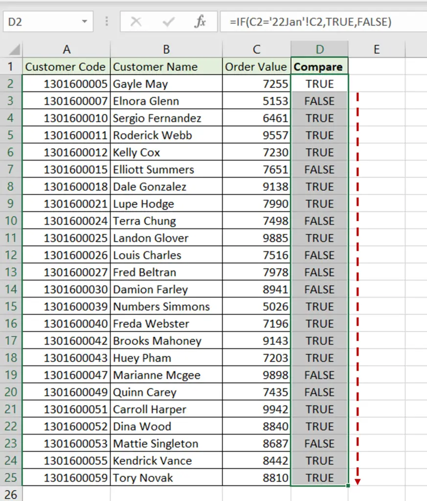
- Using the fill handle from the first cell, drag the formula to the remaining cells
OR
- Select the cell with the formula and press Ctrl+C or choose Copy from the context menu (right-click)
- Select the rest of the cells in the column and press Ctrl+V or choose Paste from the context menu (right-click)
Step 4 – Compare the values
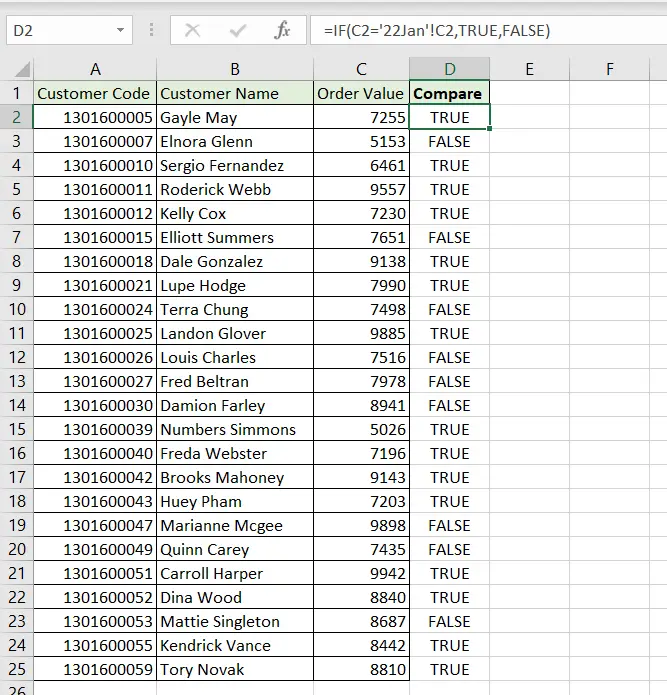
- ‘TRUE’ is displayed for the values that match and ‘FALSE’ for those that do not


