How do I color every other row in Excel

Excel is a versatile tool that can help you manage and analyze data efficiently. One of the most common tasks in Excel is formatting data to make it more readable and easier to understand. One way to do this is to Color Every Other Row in your Excel spreadsheet.

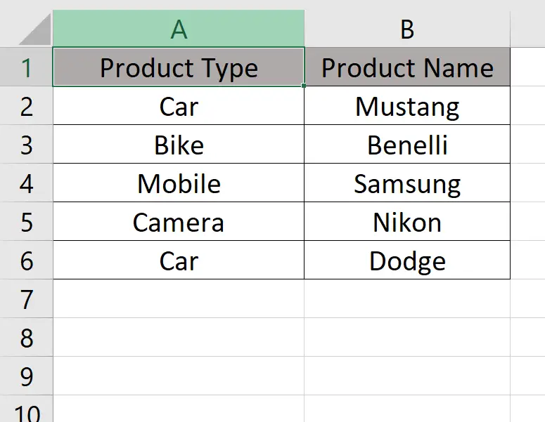
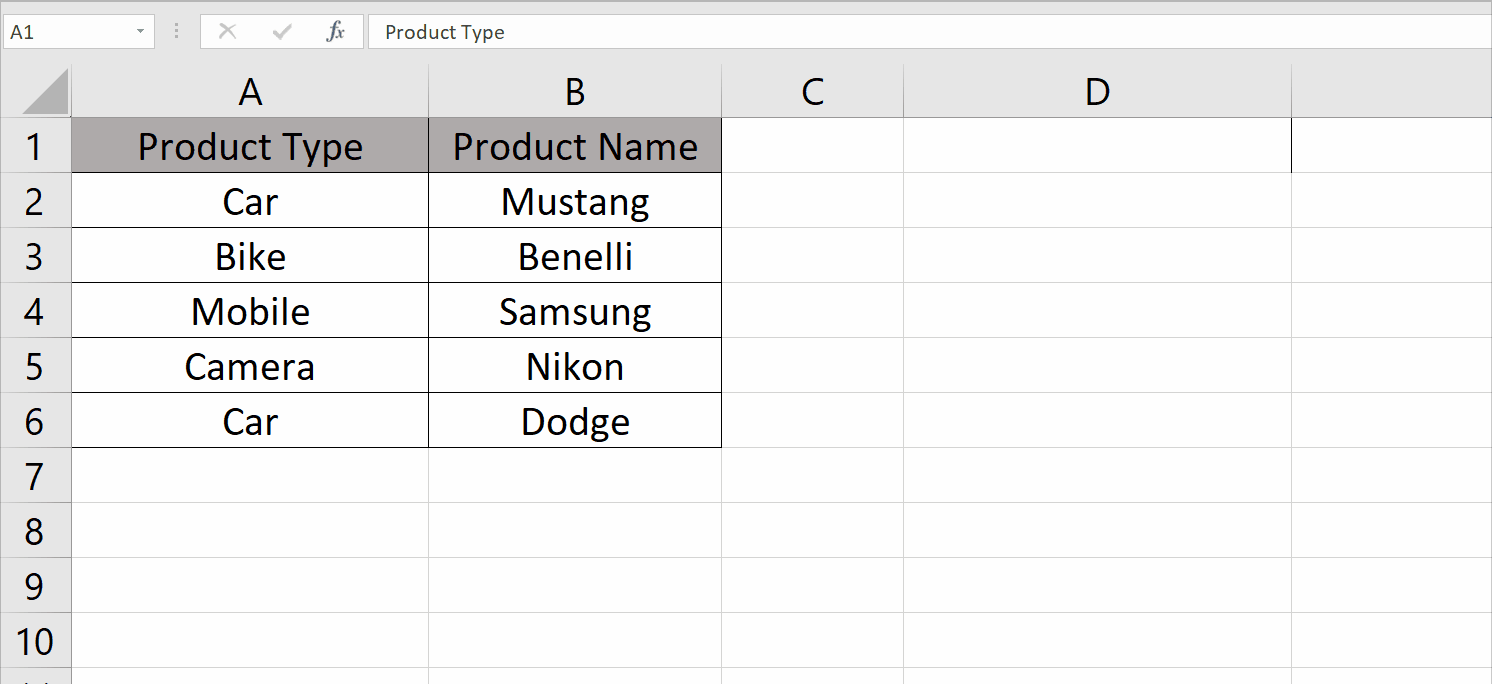
Here we have a dataset above, in this dataset, we have information regarding Product Types and their Product Names. In this tutorial, we will learn how to highlight every other row in excel to make it easier to read but first let’s take a look at the Dataset.

Method – 1 Using Conditional Formatting Formula

Step – 1 Select the Cells.

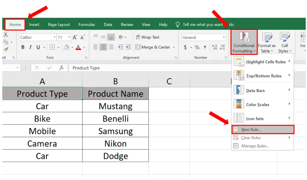
• Select the rows you want to highlight.
• Click on the Home tab.
• In the Styles group click on Conditional Formatting.
• Then in the dropdown menu click on New Rule.

Step – 2 Adding the Formula.

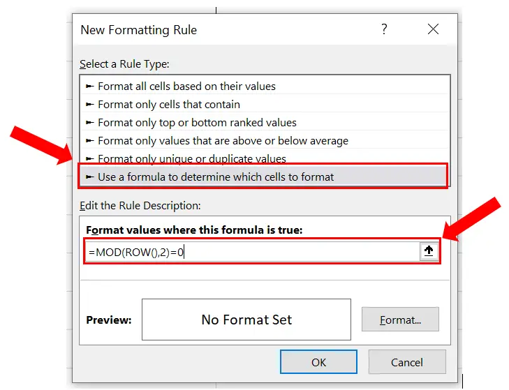
• In the New Formatting Rule dialog box click on the Use a Formula to Determine Which Cells to Format command.
• Write the formula in the Format Where this Format Is True box.
• The formula will be

=MOD(ROW(),2)=0

Step – 3 Selecting the color.

• Click on the Format button.
• Select the color from the Color dropdown menu.
• Click OK then OK again.
• The rows will be highlighted.

Method – 2 Using Branded rows.

Step – 1 Select the rows.

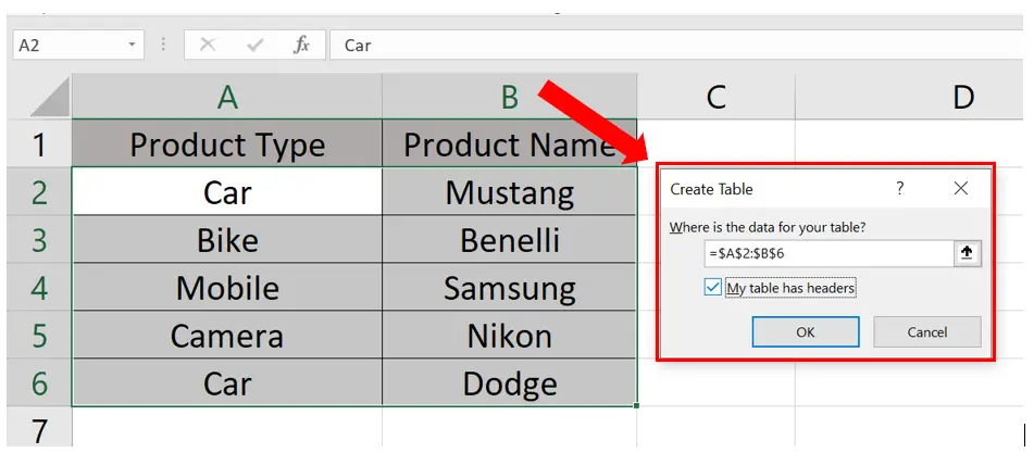
• Select the rows you want to color.
• Press Ctrl + T.
• A Create Table dialog box will appear.

Step – 2 Highlight the rows.

• In the dialog box click on My table has headers.
• Then click on OK.
• The rows will be highlighted.

Breakdown of the conditional formatting formula

The formula “=MOD(ROW(),2)=0” is used to determine whether a cell is in an even-numbered row in a worksheet.

The ROW() function returns the row number of the cell that contains the formula. The MOD() function calculates the remainder when the row number is divided by 2. If the remainder is 0, the formula returns TRUE, indicating that the row is even. If the remainder is 1, the formula returns FALSE, indicating that the row is odd.

So, if this formula is applied to a range of cells, it will return TRUE for every other row, starting from the first row in the range. For example, if the formula is applied to cells A1:A10, it will return TRUE for cells A2, A4, A6, A8, and A10, and FALSE for cells A1, A3, A5, A7, and A9.