
Highlight the row based on cell value in Excel
 By
SpreadCheaters
By
SpreadCheaters
In this tutorial, we’ll learn how to highlight specific values by a unique color within a given data range by the use of conditional formatting.
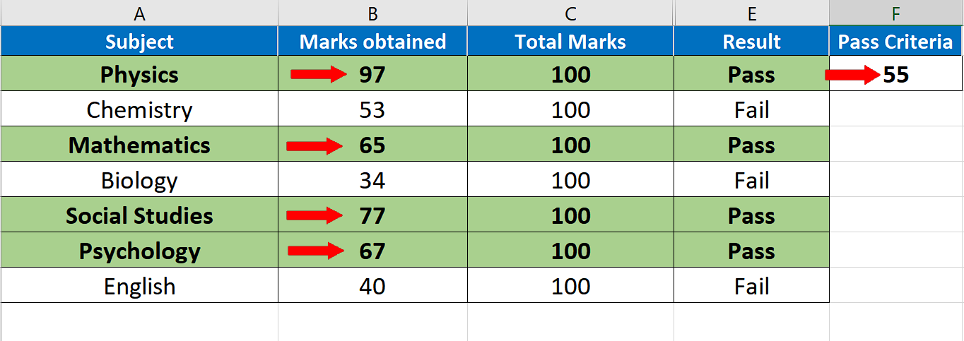
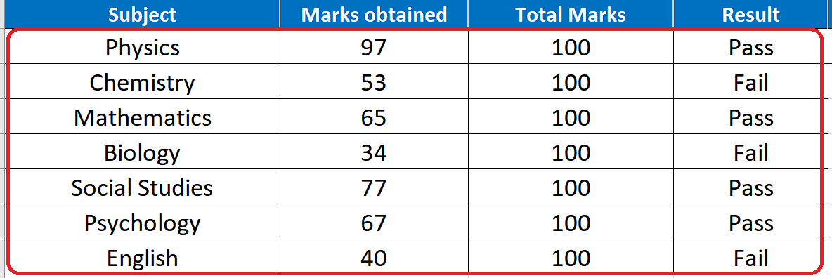
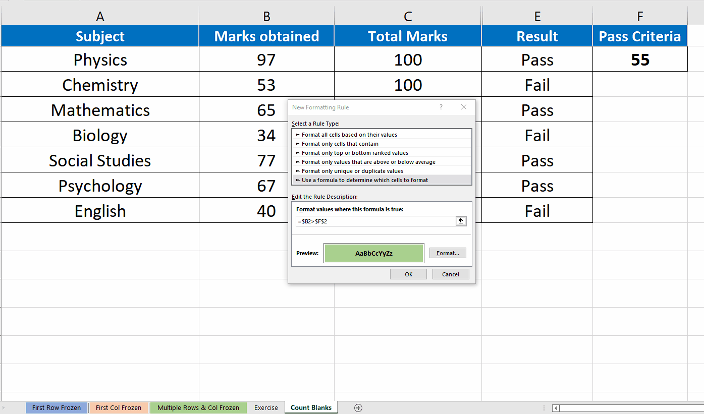
Let’s start with an example. We have a data set consisting of the details of students’ performance during exams. We want to highlight all marks that surpass a specific value in a separate cell. This cell will contain the value (55 in our example) which will decide if the student passed the subject exam or not. So let’s see how to do it.
Microsoft Excel offers incredible features to ease mathematical calculations by using built-in formulas. Along with data analysis features, it also provides us with the tools to sort, highlight and format data values to make them presentable. One of those features is the conditional formatting. It enables us to highlight the specific range of values from the entire data set.
Step 1 – Select a data range
– With the help of handle select and drag to define the data range.
Step 2 – Go to Home tab
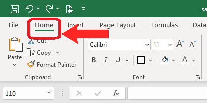
– Now go to the Home tab.
Step 3 – Go to Styles group
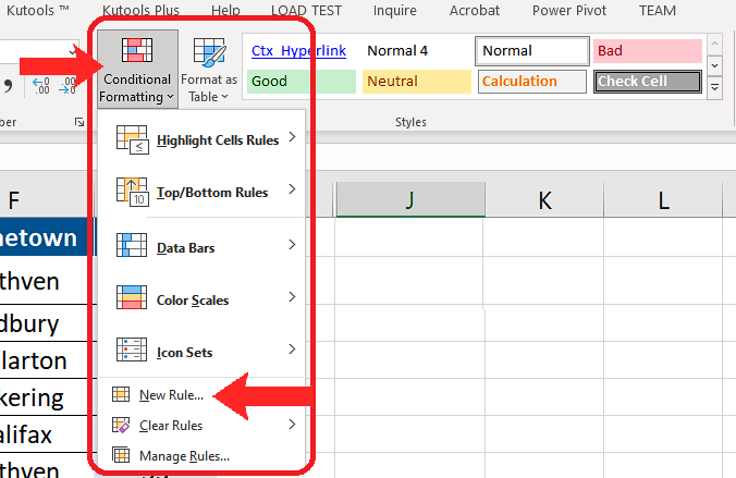
– Now go to the Styles group -> Conditional Formatting -> New Rule.
Step 4 – Write the formula to do conditional formatting
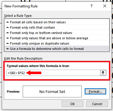
– Write the following formula in the conditional formatting formula bar;
The above formula will highlight all the cells in row 2 (i.e. complete row 2) only if the value of cell B2 is greater than cell F2. The same process will be repeated for the next row 3 and this time the formula will check the value of C3 against cell F2. The trick here is to use dollar sign ($) before Column Name B to lock the column to be checked every time the cells of any row will be analysed. Then we used the dollar sign ($) with F2 before column name F and row number 2 i.e. $F$2. This will lock the criteria cell at F2 for all rows in the selected data range.
Step 5 – Set the format for conditional formatting
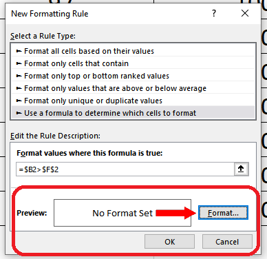
– Click on the format tab so that we can choose formatting styles to highlight our data range.
Step 6 – Set the font to bold for conditional formatting
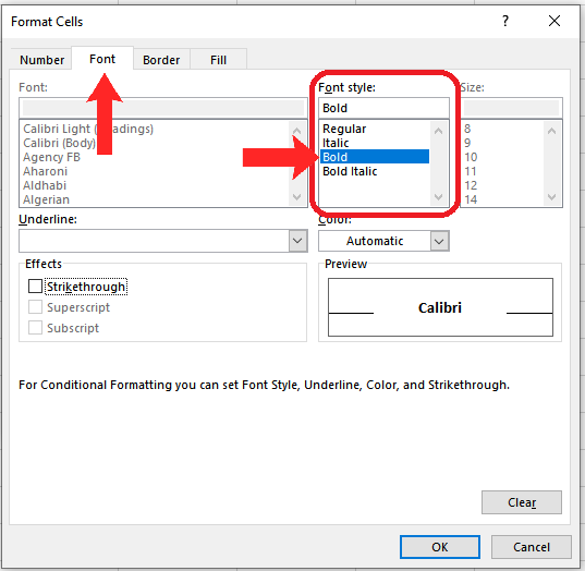
– In the next dialog box, click on the Font tab and select Bold.
Step 7 – Set the suitable colour for conditional formatting
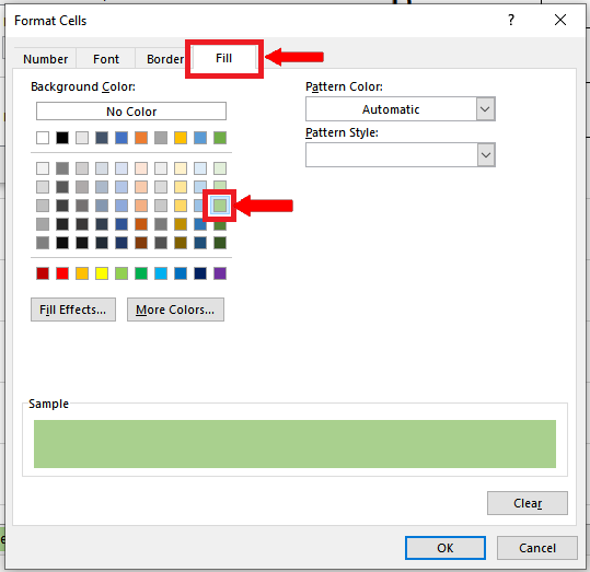
– In the same dialog box, click on the Fill tab and select an appropriate colour for highlighting the data.
Step 8 – Finalise and apply the conditional formatting settings
– When you click on the OK button in the last step, you will see the following window.
– Click on OK again. This will implement the conditional formatting rules to the selected data range.


