Google Sheets pivot table calculated field
In this tutorial, we will learn about the Google Sheets pivot table calculated field. Google Sheets offers a valuable feature known as calculated fields in pivot tables, allowing users to perform calculations directly within the pivot table using the data. This feature enhances the flexibility and functionality of the pivot table by enabling custom calculations.
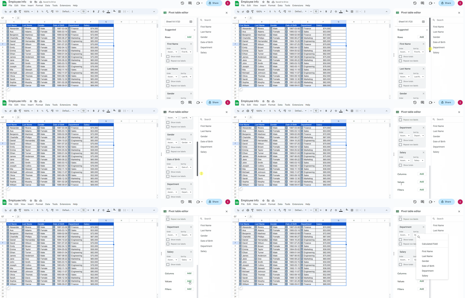
Suppose we have a pivot table containing employee details including salary. Our objective is to include a calculated field that represents the annual salary for all the employees. Below are the step-by-step instructions to achieve this.

A calculated field in Google Sheets pivot tables enables you to customize calculations on the data within your pivot table. It provides the ability to generate new fields by combining or manipulating existing fields from your data source.
Step 1 – Select the Pivot Table and Open the Pivot Table Editor

– Select the Pivot Table by selecting any cell in the table.
– An Edit button would appear at the bottom left corner of the Pivot Table.
– Perform a click on the Edit button to open the “Pivot Table Editor”.
Step 2 – Locate the Values Option

– In the menu, scroll down and locate the Values “Add” button.
– Perform a click on the “Add” button next to Values.
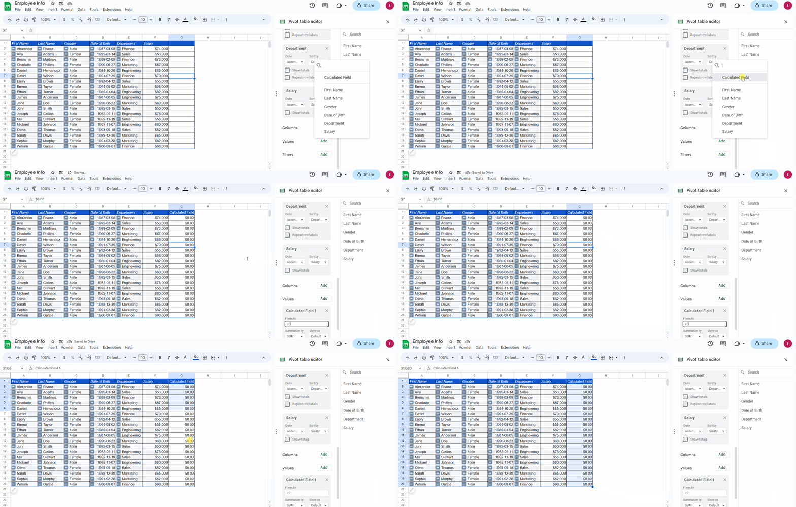
Step 3 – Choose “Calculated Feild”

– By clicking on the “Add” button, a pop-up menu will appear.
– Choose the “Calculated Feild” option in the menu.
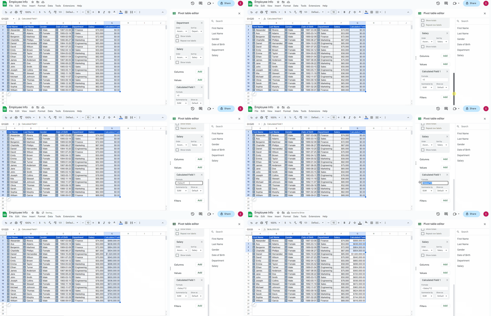
Step 4 – Insert the Formula

– Insert the formula to add the calculated field.
– In this case, we want to calculate the annual salary so we will simply multiply salary by the number 12.
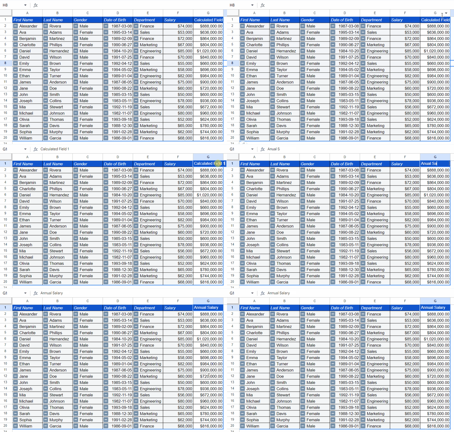
Step 5 – Rename the Calculated Feild

– Rename the “Calculated Feild” by editing the header.


