How to add a grand total to a pivot chart in Excel
You can watch a video tutorial here.
Assume you have a pivot chart built off a pivot table and you want to add the Grand Total to the chart to get an idea of the total number. If you add the Grand Total as a part of the chart, it will throw the visualization off balance as the number will be much greater than all the others. Instead, it is better to add it as a separate field that will get updated when filters are applied.
Grand Totals cannot be added directly to the Pivot chart. In this example, we will create a reference field for the Grand Total and link it to a text box placed in the chart. We cannot link the text box directly to the Pivot table.
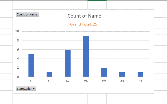
Pivot tables are one of the most useful tools in Excel for summarizing and analyzing data. Pivot charts are created from Pivot tables. Instead of using the raw data source for the chart, Pivot charts are built off Pivot tables and present a visualization of the pivot table. Pivot tables contain a Grand Total which does not get displayed in the pivot chart by default.
Step 1 – Create a reference for the Grand Total
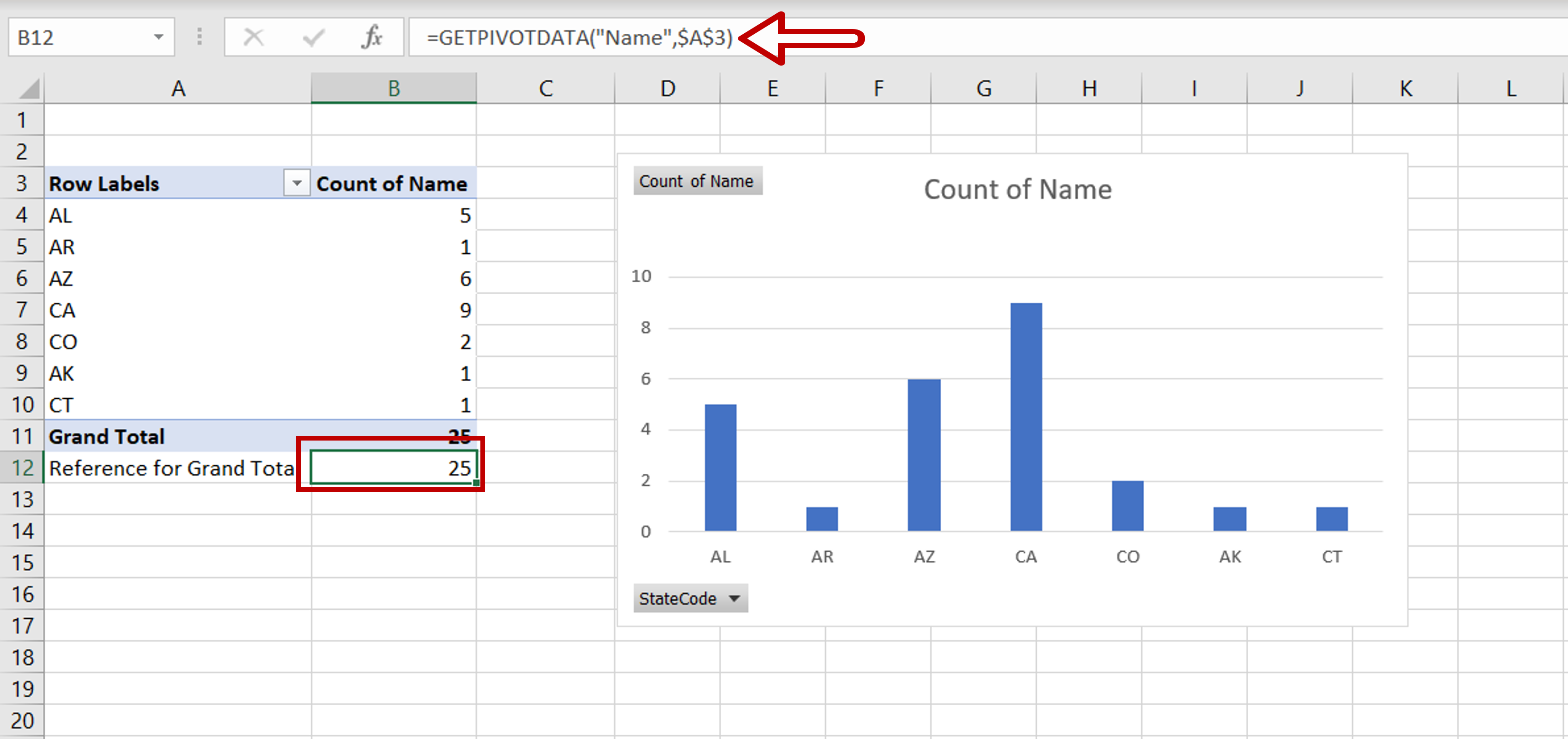
– Select any cell below the pivot table
– Type: =
= Click on the Grand Total of the pivot table
– The GETPIVOTDATA formula will automatically be populated in the cell
Step 2 – Enhance the formula by adding text
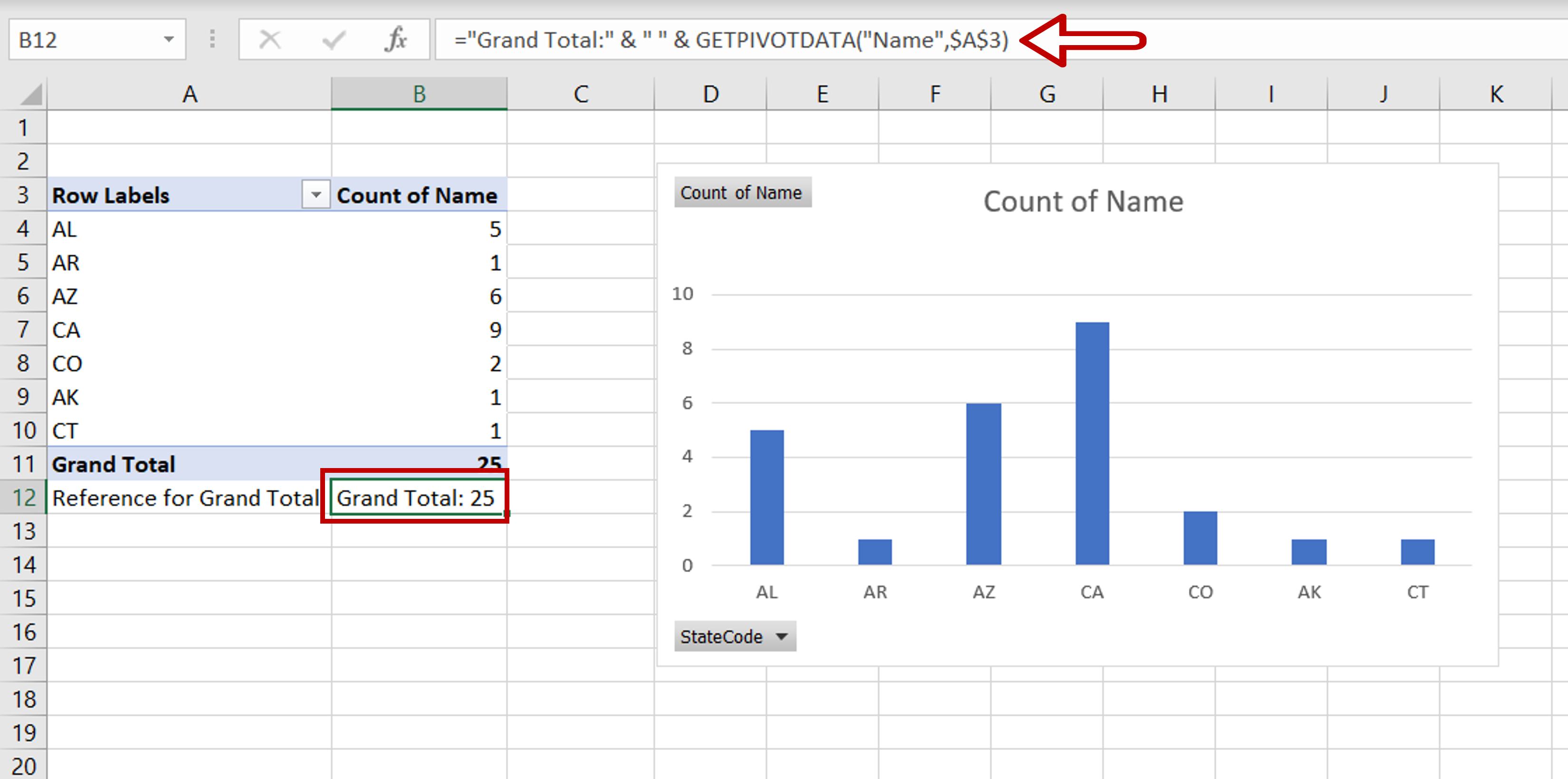
– Add text to the reference cell by typing:
= “Grand Total: “ & “ “ & GETPIVOTDATA formula
– This concatenates the text, a space, and the formula so that the number displayed will have a label
Step 3 – Create a text box
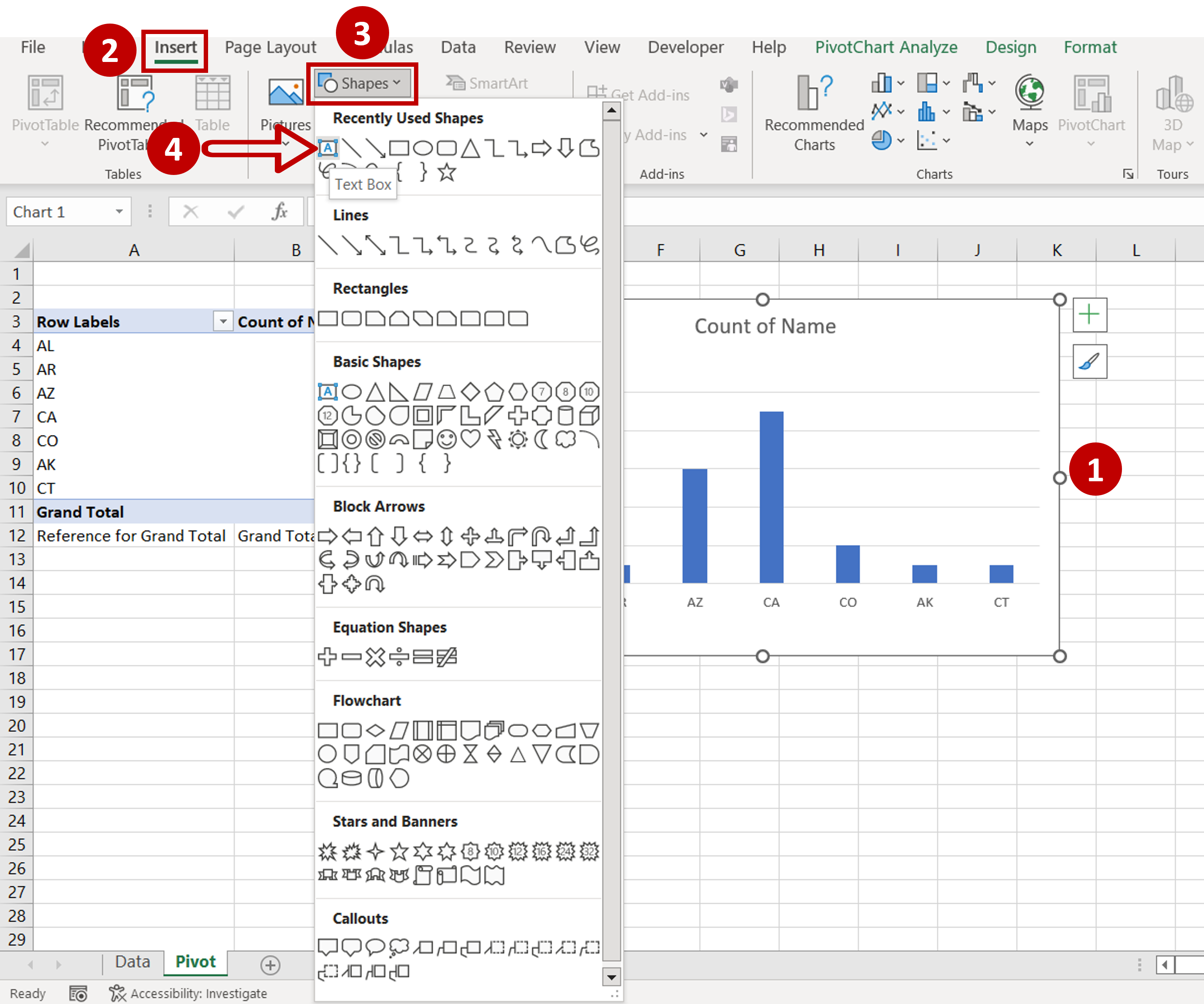
– Select the chart
– Go to Insert > Illustrations > Shapes
– Click on the Text box
Step 4 – Create the formula in the text box
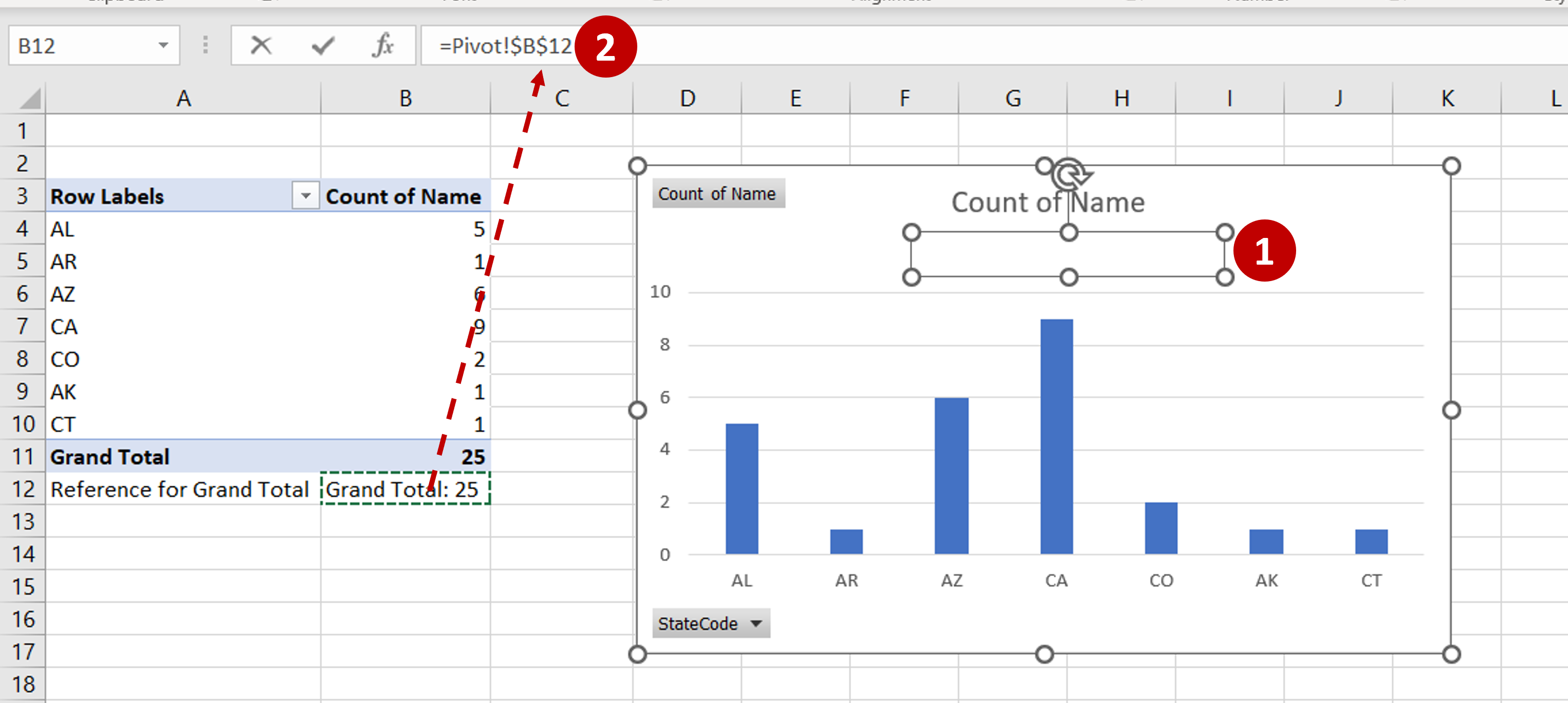
– Draw the text box within the chart
– With the text box selected, in the formula bar type: =
– Select the reference cell that has the GETPIVOTDATA formula
Step 5 – Check that the Grand Total gets updated with filters
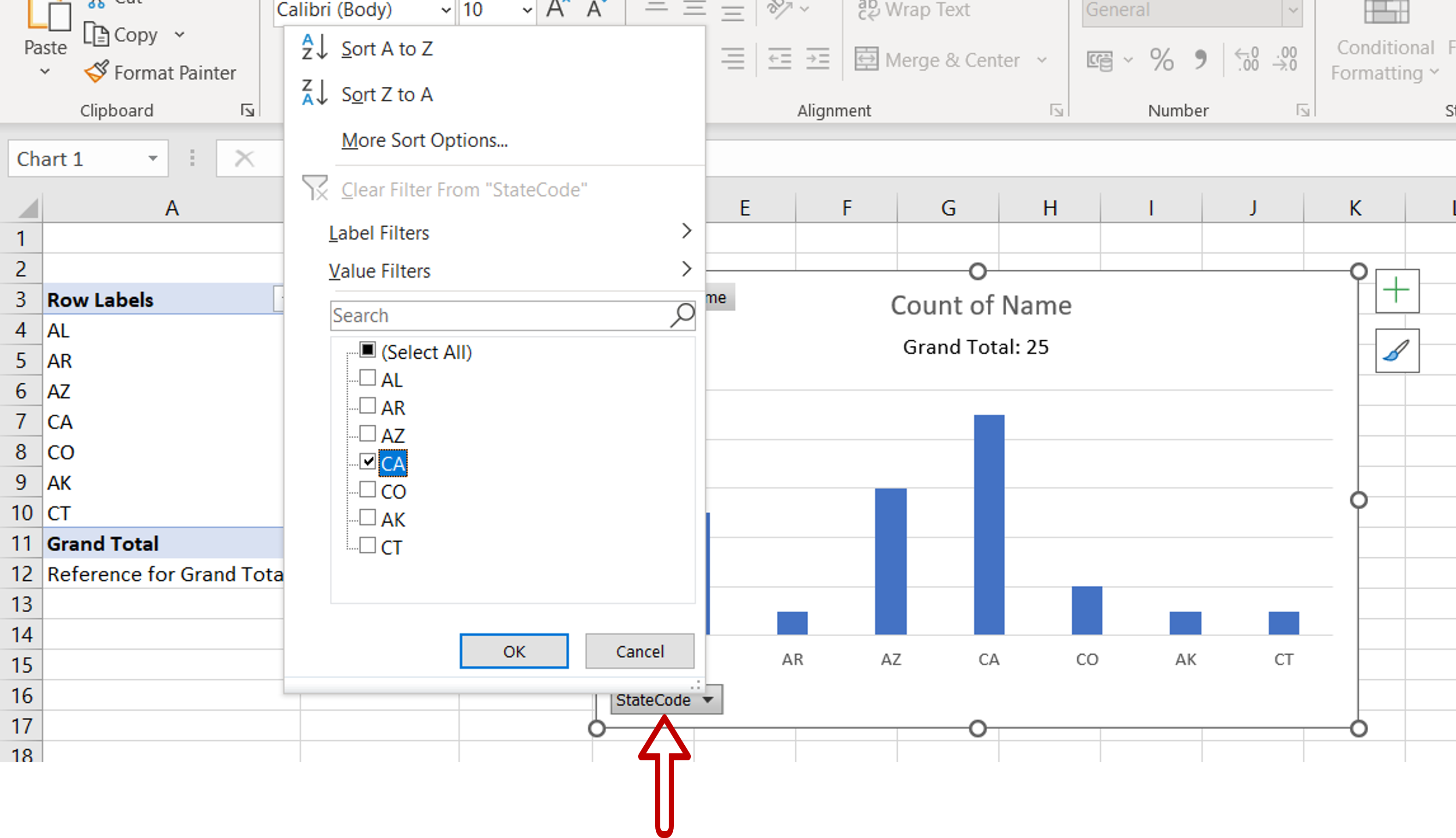
– From the State code filter, select ‘CA’
– Click OK
Step 6 – Check the result
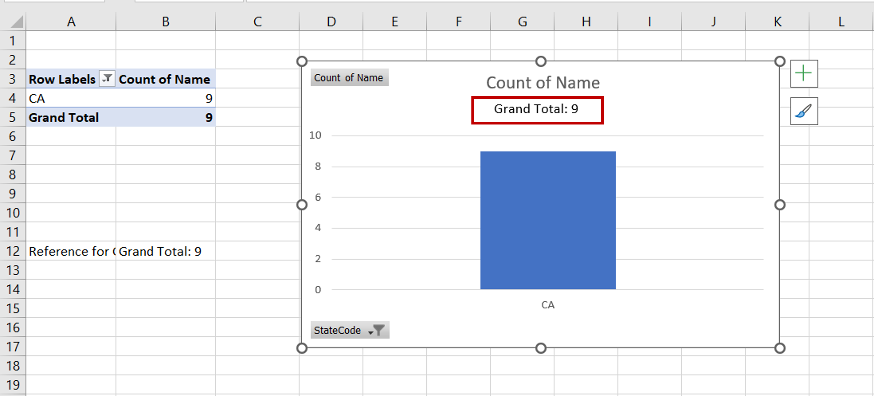
– The Grand Total gets updated when the filter is applied


