
How to change horizontal axis value in Excel
 By
SpreadCheaters
By
SpreadCheaters
Page last updated:
04/11/2022 |
Next review date:
04/11/2024
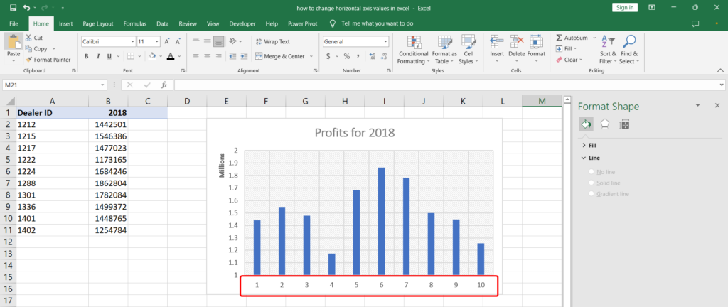
While excel has a lot of cool features for charts and graphs, sometimes we may need to change axis values after the chart has been created. Let’s see how we can do that.
Step 1 – Select Data button
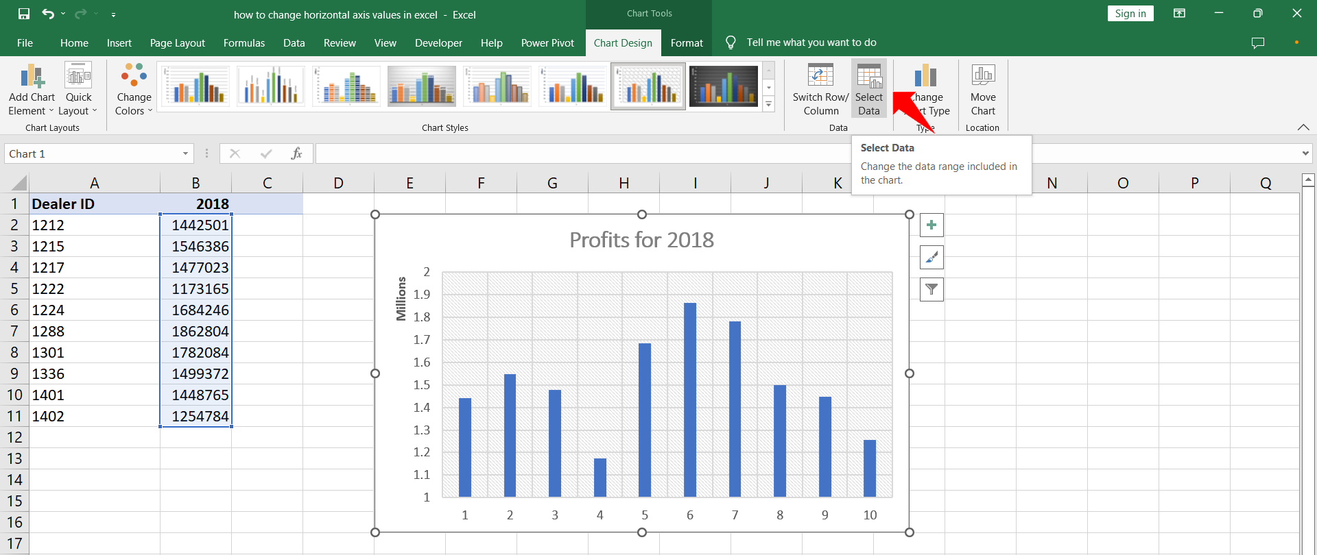
– Click the chart. The Chart Tools will appear in the ribbon.
– Click the Chart Design tab.
– In the Data group click the Select Data button.
Step 2 – Select Data Source dialog

– On clicking the Select Data button the Select Data Source dialog box will appear on screen.
– Under the Horizontal (Category) Axis Labels click Edit.
– Axis Labels dialog will appear.
– Under the Axis labels range:, click the textbox labeled Select Range.
– Click and drag to select the Dealer ID values from cells A2 to A11.
– Click OK and then OK again.
– The horizontal axis values have been changed.


