
How to reverse numbers in Excel
 By
SpreadCheaters
By
SpreadCheaters
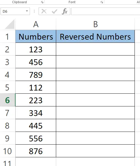
Here we have a sample dataset that contains random numbers. In this tutorial, we will learn how to reverse the order of the number in each cell in Excel by following the steps below. Let’s have a look at the dataset first above.

Excel is a powerful tool for organizing, analyzing, and visualizing data. One common task in Excel is reversing numbers, which can be useful for various applications, such as sorting data or creating number sequences.
Step 1 – Type the Formula
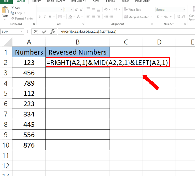
– Select the cell where you want to type the formula.
– Formula we used is:
=RIGHT(A2,1)&MID(A2,2,1)&LEFT(A2,1)
The formula explanation is given in the last.
Step 2 – Find values for the rest of the cells
– Select the cell with formula.
– Drag that cell from bottom right to the rest of the cells.
– Values for the rest of the cells will appear automatically.
Formula Explanation:
RIGHT (text,num_chars)&MID(text,start_num,num_chars)& LEFT(text,num_chars)
This formula will rearrange the characters in cell A2 to reverse the order of the first and last characters.
The RIGHT function with an argument of 1 returns the rightmost character of the text string in cell A2.
The MID function with arguments of 2 and 1 returns the second character of the text string in cell A2.
The LEFT function with an argument of 1 returns the leftmost character of the text string in cell A2.
So, if cell A2 contains the text string “hello”, the formula will return “oellh”, which is the result of taking the rightmost character “o”, the second character “e”, and the leftmost character “h” and concatenating them in reverse order.


