
How to remove numbers in Excel from the left
 By
SpreadCheaters
By
SpreadCheaters
Microsoft Excel is a powerful spreadsheet application that is widely used for organizing, analyzing, and presenting data. One common task that users often need to perform in Excel is removing numbers from a cell’s contents. This can be useful when dealing with large datasets that have extraneous information at the beginning of each cell.
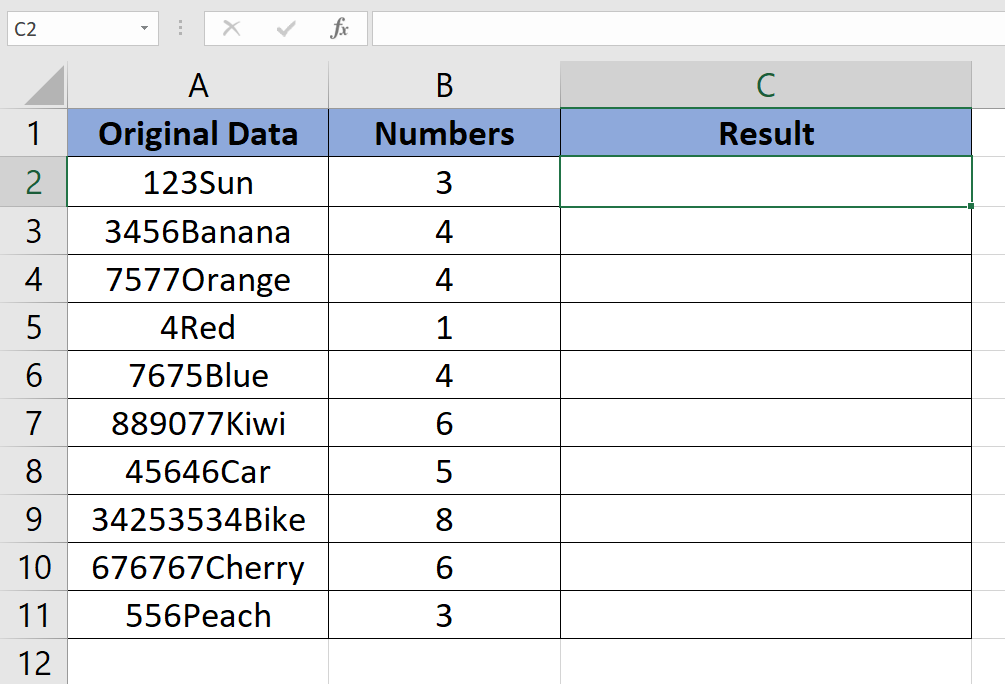
Here we have a random dataset, in this dataset above, there are some useless numbers at the beginning of the Original Data column and Numbers columns which represent the number of digits that need to be removed. If this columns is not available in your dataset then you will have to add this column yourself to make things easy. In this tutorial, we will learn how to remove these numbers using a method in the Result column by following the steps below.
Method 1: Using the RIGHT and LEN Formula.
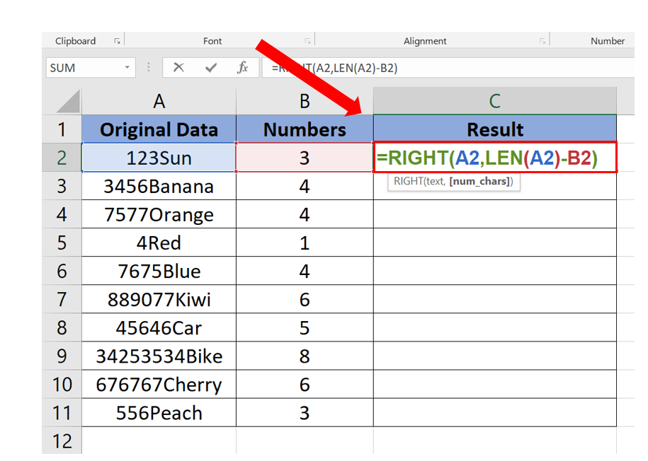
Step 1 – Type the RIGHT and LEN Formula.
- Select the cell where you want to type the Formula.
- Syntax of the formula will be
=RIGHT(First_Cell_Address,LEN(First_Cell_Address)-Num_Chars_Cell)
- In our case formula will be
=RIGHT(B5,LEN(B5)-C5)
Step 2 – Find values for the rest of the cells.
- Select the cell with the formula.
- Drag the cell from the bottom right to the rest of the cells.
- Formula will be applied automatically.
Method 2: Using the REPLACE Formula.
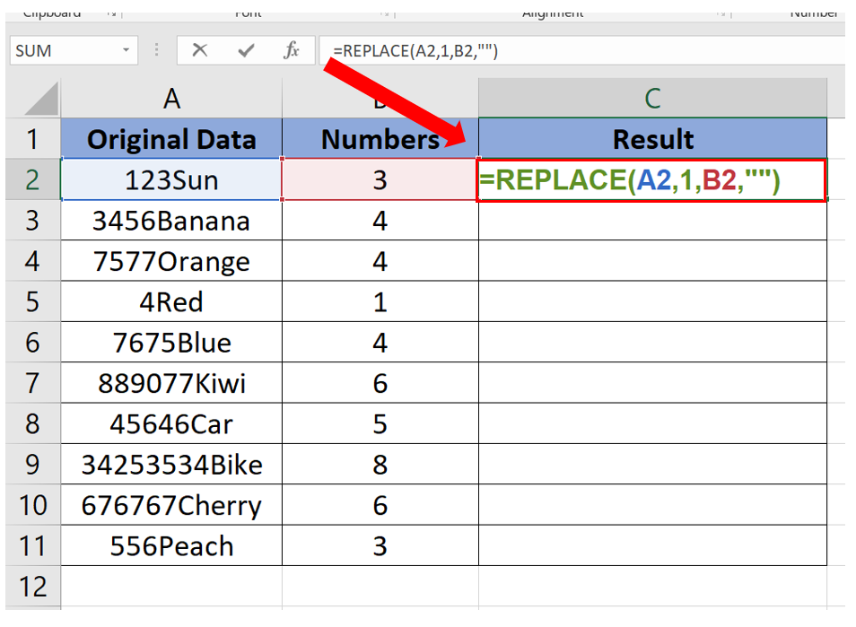
Step 1 – Type the REPLACE formula.
- Select the cell where you want to type the formula.
- Syntax of the formula will be
=REPLACE(Cell_Address,Start_Of_Range,Num_Chars, “Value_To_Replace_With”)
- In our case the formula will be
=REPLACE(A2,1,B2,””)
Step 2 – Finding values of the rest of the cells.
- Select the cell with the formula.
- Drag the cell from the bottom right to the rest of the cells in the column.
- The formula will be applied automatically.


