
How to highlight two different columns in Excel
 By
SpreadCheaters
By
SpreadCheaters
Page last updated:
13/01/2023 |
Next review date:
13/01/2025
You can watch a video tutorial here.
Excel provides several options for formatting cells. You may want to draw the reader’s attention to particular pieces of information on a sheet by highlighting a column. To do this, you can change the background color of the cell so that it stands out. When you need to highlight two adjacent columns, you can select the columns and then highlight them by changing the background color of the cell. In this example, we will see how to highlight two columns that are not adjacent to each other.
Option 1 – Use the button on the ribbon
Step 1 – Select the first column

- Select the top cell in the first column to be selected
- Press Ctrl+Shift+Down arrow
- The data in the column is selected
Step 2 – Select the second column

- Hold down the Ctrl key
- Click on the top cell in the second column
- Press Shift+Down arrow
Step 3 – Choose a color
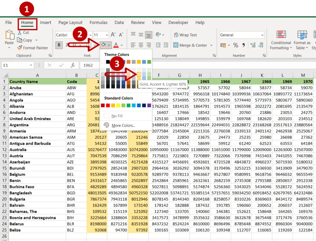
- Go to Home > Font
- Expand the Fill Color dropdown
- Select a color
Step 4 – Check the result

- The selected columns are highlighted
Option 2 – Use the Format Cells window
Step 1 – Select the first column

- Select the top cell in the first column to be selected
- Press Ctrl+Shift+Down arrow
- The data in the column is selected
Step 2 – Select the second column

- Hold down the Ctrl key
- Click on the top cell in the second column
- Press Shift+Down arrow
Step 3 – Open the Format Cells window
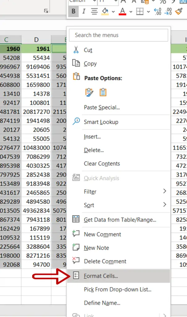
- Right-click and select Format Cells from the context menu
OR
Go to Home > Number and click on the arrow to expand the menu
OR
Go to Home > Cells > Format > Format Cells
OR
Press Ctrl+1
Step 4 – Choose a color
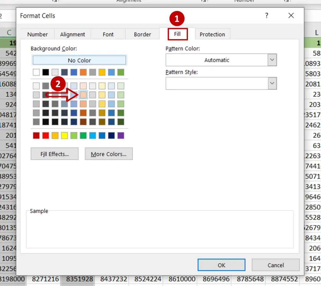
- Go to the Fill tab
- Select a color
- Click OK
Step 5 – Check the result

- The selected columns are highlighted


