
How to calculate the correlation coefficient in Excel
 By
SpreadCheaters
By
SpreadCheaters
Page last updated:
05/01/2023 |
Next review date:
05/01/2025
You can watch a video tutorial here.
The correlation coefficient is a metric that measures the relationship between 2 datasets. In Excel, this can be done using the data analysis tool or by using the CORREL() function.
- CORREL(): this returns the correlation coefficient of 2 sets of data
- Syntax: CORREL(array1, array2)
- Array1: the first dataset
- Array1: the second dataset
- Syntax: CORREL(array1, array2)
Option 1 – Use the Data Analysis tool
Note: If the Data Analysis button is on the Data > Analyze ribbon, then skip Steps 1 to 3 below.
Step 1 – Open the Excel Options window

- Go to File > Options
Step 2 – Manage the Add-ins
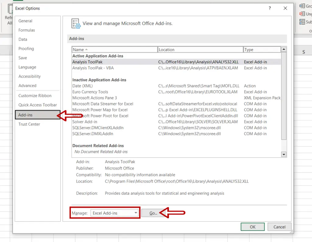
- Go to Add-ins
- Select Excel Add-ins from the Manage drop-down
- Click Go
Step 3 – Load the Analysis ToolPak add-in
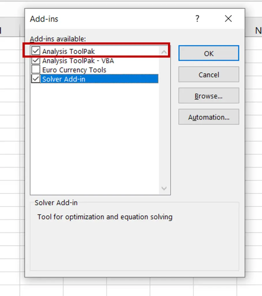
- Select Analysis ToolPak
- Click OK
Step 4 – Open the Correlation window
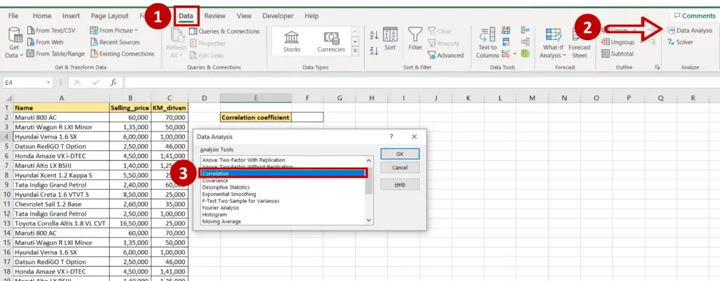
- Go to Data > Analyze
- Click on the Data Analysis button
- In the window, select Correlation
- Click OK
Step 5 – Set the parameters
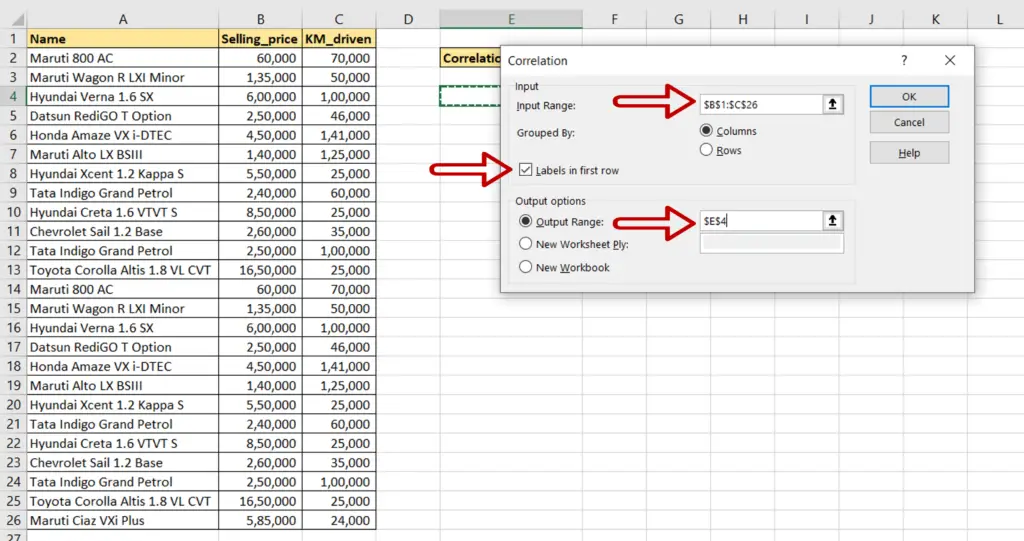
- Define the input range:
- Input Range: the range of both the ‘Selling Price’ and ‘KM_driven’ columns
- Tick the Labels in first row box
- Output Range: the location where the result is to be displayed
- Click OK
Step 6 – Check the result
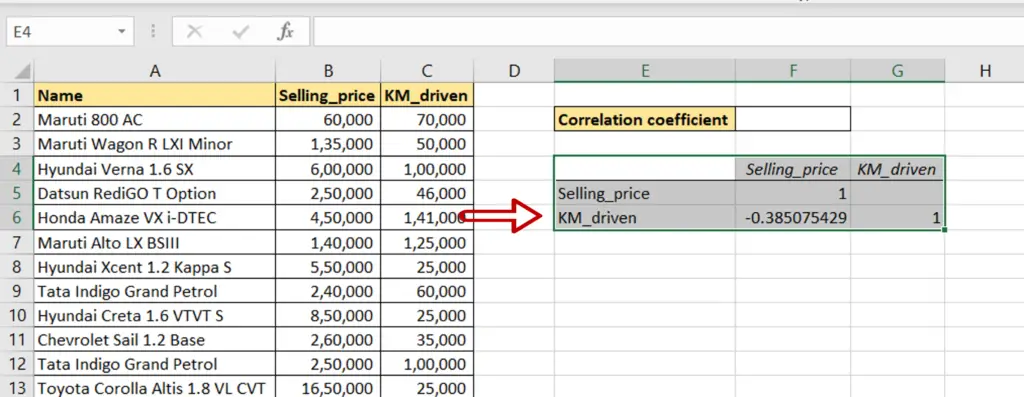
- The correlation coefficient between the variables is displayed
Option 2 – Use the CORREL() function
Step 1 – Create the formula
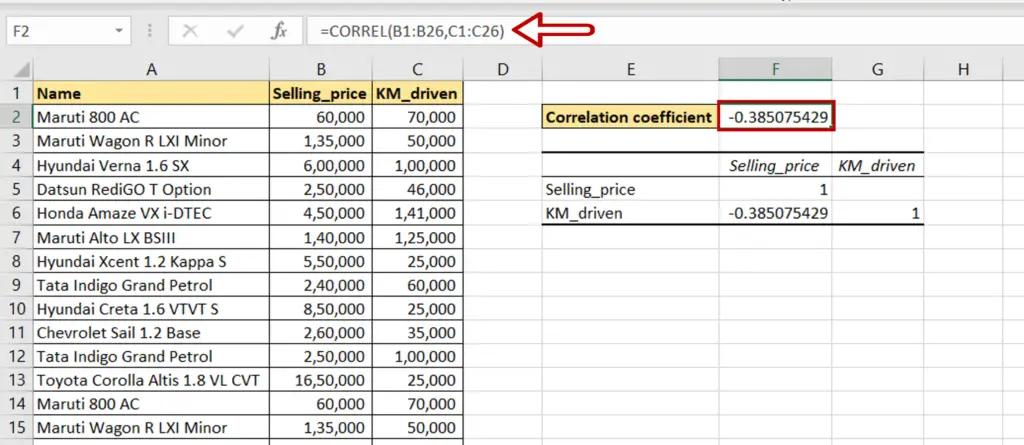
- Select the cell where the result has to be displayed
- Type the formula using cell references:
=CORREL(range of Selling_price, range of KM_driven)
- Press Enter
Step 2 – Check the result
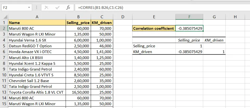
- The correlation coefficient is displayed


