
How to pull text from a cell in Excel
 By
SpreadCheaters
By
SpreadCheaters
You can watch a video tutorial here.
Excel has several functions that can be used to manipulate text. Some of these functions can be used to pull text from a cell. Text extracted from a cell is known as a substring. When working with data, you may need to pull certain text from a cell or split the text in a cell to make the data more granular.
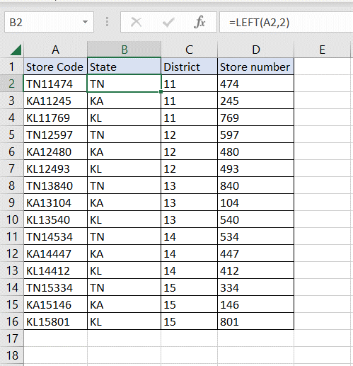
In this example, we have a store code in which the first 2 characters are the state, the next 2 are the district and the last 3 are the store number. We will use the following functions to pull the state, district, and store number from the cell:
1. LEFT() function: this returns a specified number of characters from the left of a string
a. Syntax: LEFT(text, number of characters)
i. text: the string from which the characters are to be extracted
ii. number of characters: the number of characters to extract
2. RIGHT() function: this returns a specified number of characters from the right of a string
a. Syntax: RIGHT(text, number of characters)
i. text: the string from which the characters are to be extracted
ii. number of characters: the number of characters to extract
3. MID() function: this returns a specified number of characters from a string
a. Syntax: MID(text, start number, number of characters)
i. text: the string from which the characters are to be extracted
ii. start number: the number of the character from which the extraction is to start
iii. number of characters: the number of characters to extract
Step 1 – Pull the ‘State’
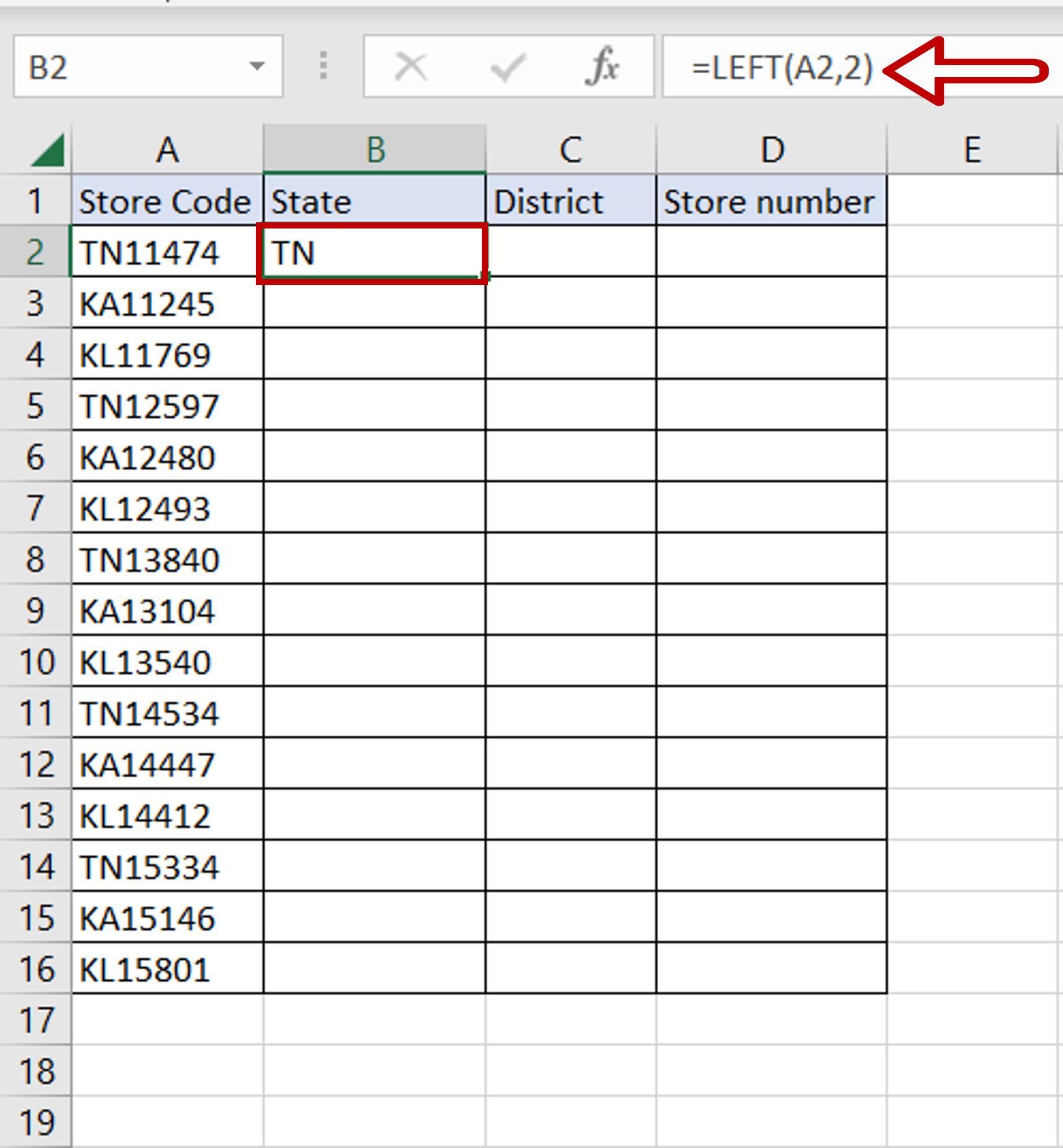
– Go to the first cell of the ‘State’ column
– Type the formula using cell references:
=LEFT(Store Code,2)
– Press Enter
– The first 2 characters i.e. the ‘State’ code are pulled from the cell
Step 2 – Pull the ‘Store number’
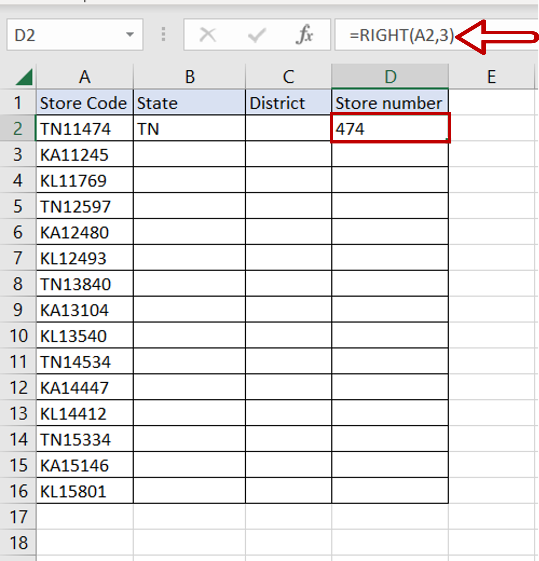
– Go to the first cell of the ‘Store number’ column
– Type the formula using cell references:
=RIGHT(Store code, 3)
– Press Enter
– The last 3 characters i.e. the ‘Store number’ are pulled from the cell
Step 3 – Pull the ‘District’
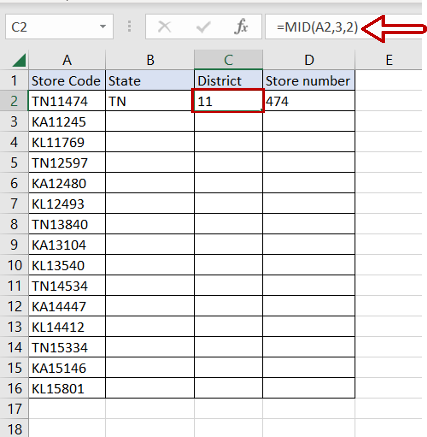
– Go to the first cell of the ‘District’ column
– Type the formula using cell references:
=MID(Store code, 3,2)
– The code for the district starts at the 3rd character and consists of 2 characters
– Press Enter
– The middle 2 characters i.e. the ‘District’ are pulled from the cell
Step 4 – Copy the formula
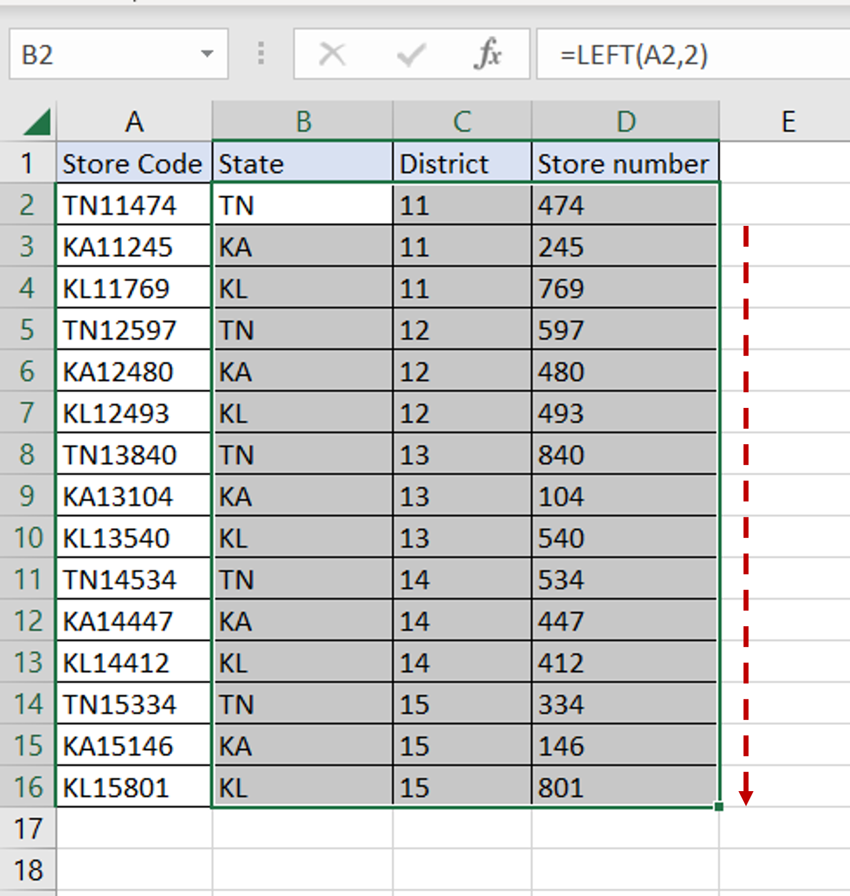
– Select the 3 formulas that have been created in the previous steps
– Using the fill handle from the selection, drag the formula to the remaining cells
OR
a) Select the cells with the formulas and press Ctrl+C or choose Copy from the context menu (right-click)
b) Select the rest of the cells in the columns and press Ctrl+V or choose Paste from the context menu (right-click)
Step 5 – Check the result
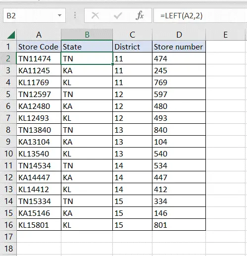
– Text representing the State, District, and Store number has been pulled from the cell


