
How to use named ranges in Google Sheets
 By
SpreadCheaters
By
SpreadCheaters

Named ranges in Google sheets or Excel play a very important role in making it easier to understand the purpose of a range of cells. Especially, if you have a large and complex spreadsheet then using named ranges wisely and appropriately makes the data easy to understand and refer to various ranges in formulas by using their names instead of using the actual range values.
In this tutorial we’ll see how to create name ranges and then use them in formulas for calculations.
Step 1 – Select the data range and create a named range
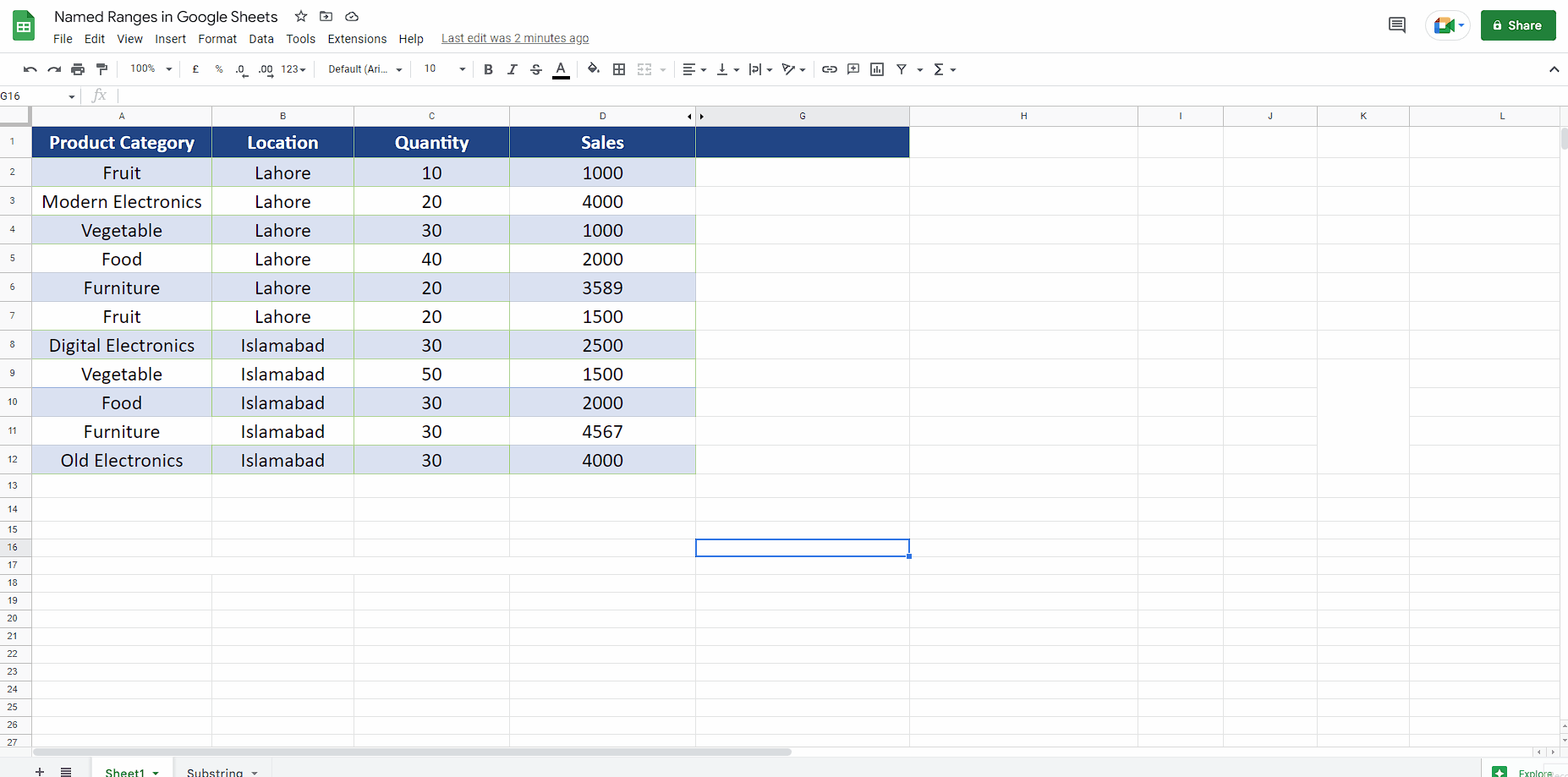
– Select the data range for which you wish to create a named range.
– On the main list of tabs click on the Data tab and select Named ranges.
– This will open up a sidebar. Choose an appropriate name for the data range, we’ll use “Lahore” and “Islamabad” for two named ranges.
– Click the Done button after writing the names in appropriate fields. This will create the named ranges as shown above.
Step 2 – Use a named range in the formula
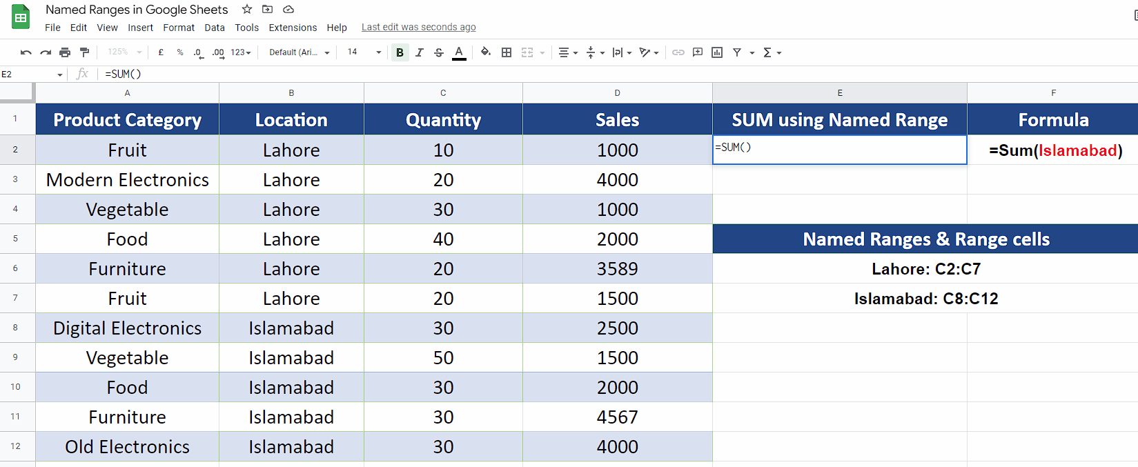
– After creating a named range, we can use it in the formulas very easily for example SUM, MAX, MIN and AVERAGE etc. We’ll use the named range to calculate the subtotal from the sales data.
– We’ll use the named ranges Lahore and Islamabad to calculate the SUM of the number of items sold from each location for the sake of explaining the method to use the named ranges. However, you can use the named ranges in many other ways as well as per your own requirements.


