Google Sheets is probably one of the best online tools which is nearly an exact alternate solution to Microsoft Excel. It has myriad features to handle, manipulate and perform simple to complex calculations on any type of dataset. 

INDIRECT function may look straightforward to use but it has many dimensions when it is used along with other formulas. In today’s tutorial we are going to learn how to use the INDIRECT function in Google Sheets directly and with the combination of other functions as well.

• INDIRECT to create a fixed reference
• INDIRECT to refer to a variable sheet name
• INDIRECT with SUM using the named ranges
• INDIRECT with VLOOKUP

Before jumping directly to the usage of this formula, let’s understand the purpose and syntax of this formula first.

Syntax of the formula

The syntax of this function is as follows;

INDIRECT(ref_text, [ref_style])

The function takes two parameters:

• ref_text: This is a text string containing a reference to a cell or range of cells or a named range as well.
• [ref_style]: This parameter is optional. It is specified with a TRUE/ FALSE value. A TRUE value indicates that the ref_text is specified in “A1” notation, while a FALSE value indicates that it is specified in the “R1C1” notation. If this value is not specified, the default value is assumed to be TRUE.

Now let’s dive into the ways INDIRECT can be used in Google Sheets.

Example 1: INDIRECT to create a fixed reference to a cell or range of cells

The best and easiest use of INDIRECT is to create a fixed reference that will not change even when cells, rows, or columns are inserted or deleted. For example, the reference created through INDIRECT to the first 10 rows of column A, will never change even if rows in that range are deleted or inserted. Let’s see how to do it in the following steps.

Step 1 – Create a reference using INDIRECT

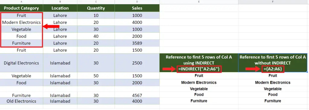
• We’ll use the following formula to create a reference to the range A2:A6 using the following formula with INDIRECT.

=INDIRECT(“A2:A6”)

• We’ll also create another reference using the normal reference through direct reference to the range using the following formula

={A2:A6}

Step 2 – Insert two rows in the reference range

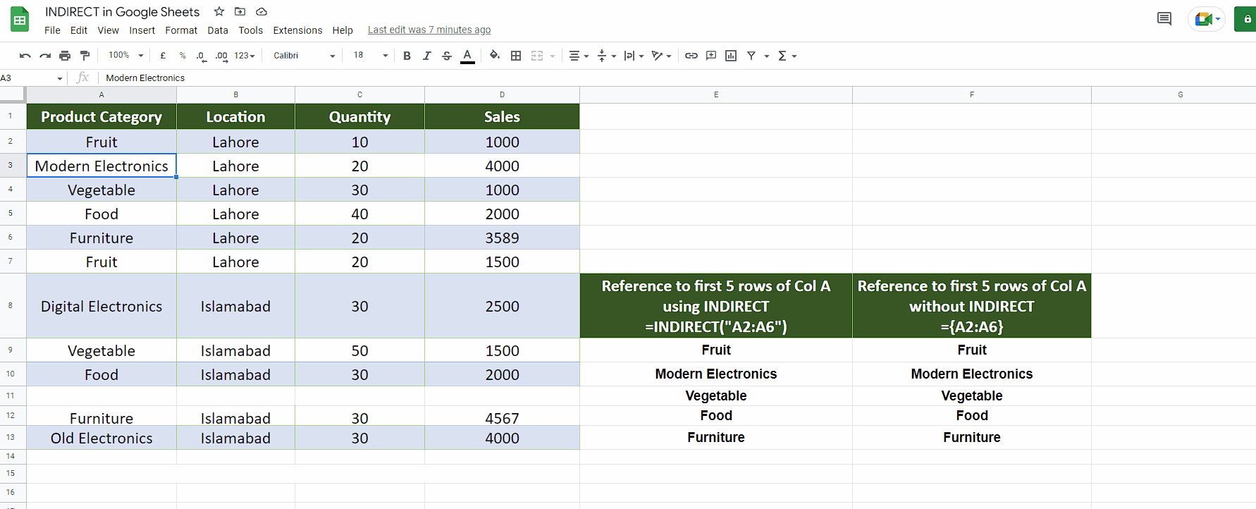
• Initially both results from the two formulas used in the first step look the same. Now we’ll insert two rows and see the effect on both formulas. Select the first two rows from the row index numbers.
• Right click and open the context menu. Now choose the option insert two rows above.
• This will insert two new rows in the reference range. Now we’ll see that the results from both formulas have changed. The cells where we used INDIRECT were updated properly while the other range remained the same. This is because of the fact that INDIRECT always points to the same range i.e., A2:A6, while the simple reference to the range A2:A6 through = sign was changed when two new rows were added and it became A4:A8 automatically as shown above.

Example 2: INDIRECT to create a variable worksheet name

INDIRECT can also be used to create a variable worksheet name which can be used to refer to the values of cells from other sheets. Let’s see how we can do this.

Step 1 – Write sheet names in a column

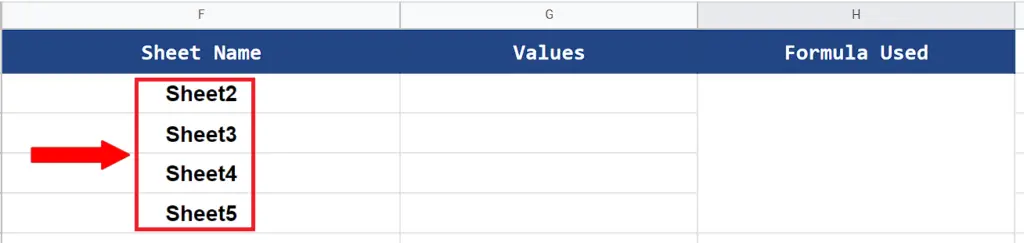
• We’ll write all the sheet names, from which we want to get the values, in a single column as shown above.

Step 2 – Create the formula with INDIRECT to get values

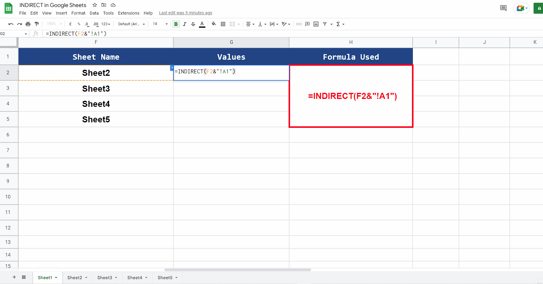
• We’ll write the following formula to combine the sheet names and cell reference to get values from all sheets.

=INDIRECT(F2&”!A1″)

• This formula concatenates the text in F2 to the string “!A1” and returns the result to INDIRECT. The INDIRECT function then evaluates the text and converts it into a proper reference and gets us the value of cell A1 from the Sheet2. Now we’ll use the fill handle to drag down the formula to fill the empty rows with values as well. The results in G2:G5 are the values of cell A1 from all sheets listed in column F as shown above.

Example 3:  INDIRECT with named ranges to calculate SUM

The INDIRECT function can easily be used with named ranges. In the worksheet below, there are two named ranges: Lahore (C2:C7) and Islamabad (C8:C12). We can enter “Lahore” or “Islamabad” in cell F2 and the formula in cell E2 will sum the respective range using INDIRECT. Let’s see how we can do it.

Step 1 – Create the formula using SUM and INDIRECT

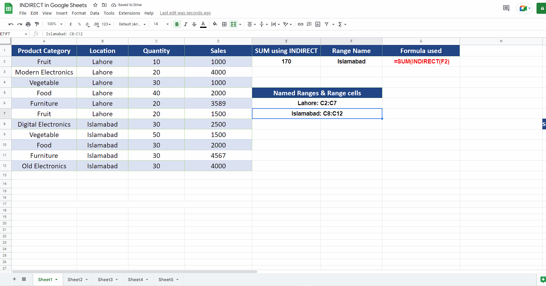
• We’ll use the following formula and it will use the named range specified in cell F2 to tell Google Sheet to use the whole range referred by that name.

=SUM(INDIRECT(F2))

• This will work on the algorithm explained above and calculate the SUM of the range specified by cell F2. To get the sum of the other range, we can write the whole formula again in the cell below or we can change the named range in cell F2 as shown above.