
How to use IFERROR in Google Sheets
 By
SpreadCheaters
By
SpreadCheaters
We often come across situations where we try to use a formula and we get an error instead of the desired result. Whether it is Microsoft Excel or Google Sheets, errors in the formulas are most likely to happen.
IFERROR is a standard Google Sheets formula which can be used to handle the common errors while using the formulas in Google Sheets.
Most Common Errors
The most common errors while using the formulas are as follows;
- #DIV/0!
- #VALUE!
- #REF!
- #N/A
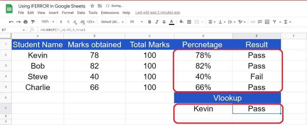
Let’s take a look at the following data set in the picture above and see which formulas are being used. We’ll intentionally create errors to understand the errors and then handle them by using IFERROR.
Example 1 – The #DIV/0! error
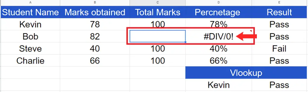
In the data sheet we have used a mathematical formula to calculate the percentage. If any data entry from total marks is deleted accidentally then we’ll get a #Div/0! error.
Example 2 – The #VALUE! Error
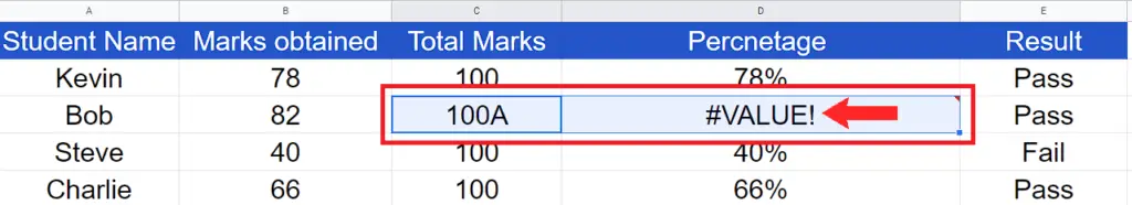
This error will be displayed when you input the wrong type of data in a formula, for example if you input text or alphabetical input where the data should be a number then you will see this error.
Example 3 – The #REF! Error
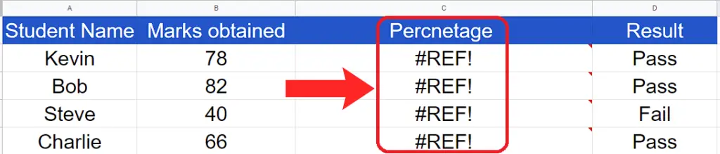
This error will occur when you delete the whole column which was used in some formula somewhere in your sheet.
Example 4 – The #N/A! Error
This error is most likely to occur when you are using the VLOOKUP function. While using VLOOKUP if the searched value is not found inside the searched range.
Syntax of IFERROR Formula
The syntax of the formula is as follows. This function requires only one input, the second argument is optional.
=IFERROR(value, [value_if_error])
value:
This is the value to be tested for errors. In most cases it is the result of a formula which is to be tested for any errors.
[value_if_error]:
This parameter is optional. If it is not used then nothing will be displayed in case of an error. However, we can use it to display meaningful messages in case of an error.
Step 1 – Implement the IFERROR formula to handle #DIV0!
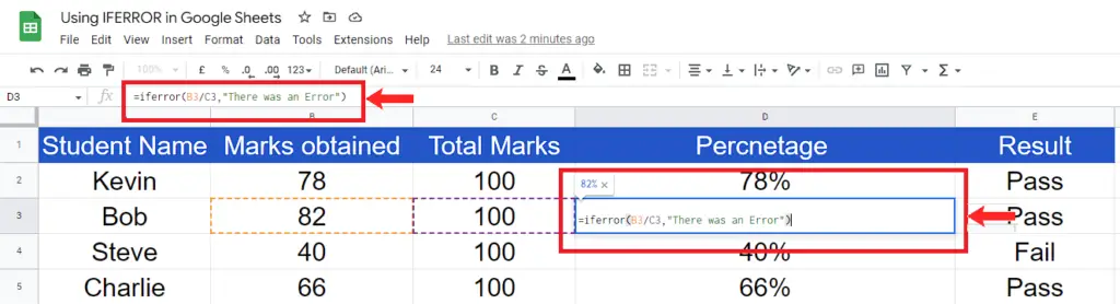
- Let’s implement this formula in the cell where we got the error to handle this error. The formula will be;
=IFERROR(B3/C3, “There was an Error”)
- Here B3/C3 is the formula to be tested for an error. We can use the same formula to capture errors from each formula and then display a meaningful message.
Step 2 – Handle #DIV/0! Error by using IFERROR
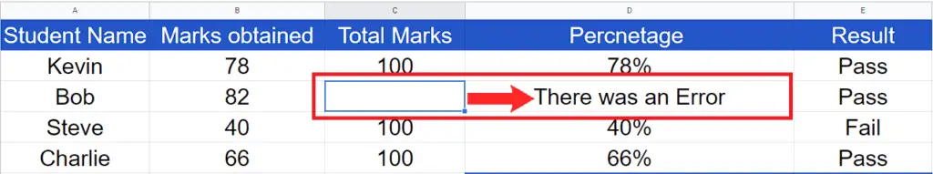
- After implementation of the formula, if we delete the value in Column C then our custom message will be displayed.
- Similarly we can use the same formula in each cell where we have used any formula.
Step 3 – Handle #N/A Error with IFERROR
- The formula to handle this error will be a little different from others. The formula will be;
=IFERROR(VLOOKUP(D7,A2:E5,5,false),“Search key is not listed”)
- We’ll get a meaningful message when the search key is not found inside the searched range.
This is how we can handle various errors using the IFERROR in Google Sheets. However, IFERROR shouldn’t be used to detect the type of error. There is another formula for that purpose which is ERROR.TYPE(reference). This can tell us which type of error has occurred. It returns an error code in case of each error which can be used to decide which type or error has occurred. However, that needs a more complex approach which is beyond the scope of this topic.


