
How to use COUNTIF with multiple criteria in Google Sheets
 By
SpreadCheaters
By
SpreadCheaters
In this tutorial we’ll learn how to use the COUNTIFS function to implement multiple criteria. For example, we’ll use COUNTIFS to count the number of times a certain product was sold from a specific location.
Syntax of COUNTIFS function
The syntax for the COUNTIFS function in Google Sheets is as follows:
=COUNTIFS(range1, criteria1, [range2, criteria2, …])
Where:
range1 is the first range of cells to be evaluated.
criteria1 is the condition to be met for cells in the first range to be counted.
[range2, criteria2, …] are optional additional ranges and criteria that can be added to further refine the count.
For example, to count the number of cells in the range A1:A10 that contain the value “apple” and the number of cells in the range B1:B10 that contain the value “red”, the formula would be:
=COUNTIFS(A1:A10, “apple”, B1:B10, “red”)
When we want to use COUNTIF with multiple criteria then Google Sheets provides us with a function COUNTIFS. This function in Google Sheets is used to count the number of cells within a specified range that meet multiple criteria. It allows you to count the number of occurrences of a specific value in multiple ranges and with different criteria.
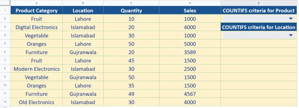
Step 1 – Create Drop-Downs for COUNTIF criteria selection
– We’ll create some drop downs from our available dataset. This will make our criteria selection dynamic. So, select the cell outside the dataset and right click.
– Choose dropdown form the context menu option.
– This will open up a sidebar of options. Locate the Criteria option and change the Drop-Down to Drop-Down (from a range).
– Click in the field below and choose the range from which you wish to create the drop-down from the Product Category column.
– Repeat the same steps for creating another drop-down for data from the Location column as shown above.
Step 2 – Create formula for COUNTIFS with multiple criteria
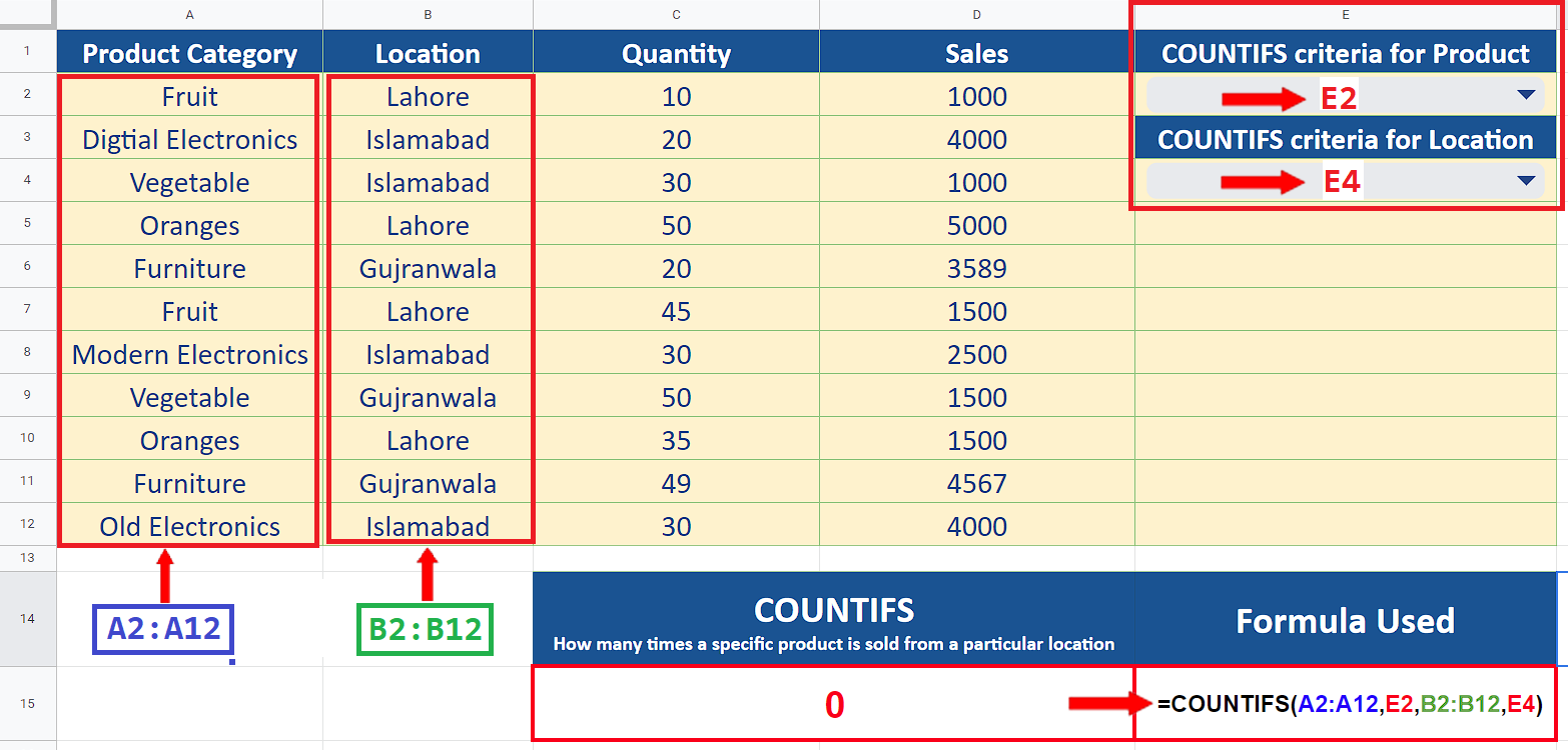
– We’ll create the formula for COUNTIFS with the newly created drop-down lists so that the selection process becomes dynamic and we can change the criteria on the go without the need of changing the formula again and again.
=COUNTIFS(A2:A12,E2,B2:B12,E4)
– In this formula A2:A12 represents the range of Products and B2:B12 is the Location range. E2 and E4 are the cells with drop-downs to select any value from Product and Location columns.
Step 3 – Implement the formula of COUNTIFS with multiple criteria

– Choose appropriate values from drop-down lists and the result of the formula will be automatically calculated. We can easily change the criteria of Product or Location. This will make our criteria selection process easy and dynamic as shown above.


