How to sum checkboxes in Google Sheets

You can watch a video tutorial here.

Google Sheets is widely used for calculations due to the several arithmetic operators and functions that it has. You can also add a checkbox in a Google Sheet that can be used to tick off an item. The value of the cell containing the checkbox evaluates to 1 if it is ticked and to zero if it is left unchecked. You can use checkboxes to indicate whether a value is to be included or not when summing the values in a column.

In this example, we have a list of items available for sale. Only those items ordered by the customer need to be included in the final bill. The items ordered are indicated by the checkboxes that are ticked. To do this, we will make use of the ARRAYFORMULA() and SUM() functions.

1. SUM() function: this returns the sum of a range of numbers or individual numbers
   1. Syntax: SUM(numbers)
      1. numbers: this is a range of numbers or individual ranges/numbers separated by a comma
2. ARRAYFORMULA() function: this allows you to use a formula across a range of cells
   1. Syntax: ARRAYFORMULA(array formula)
      1. Array formula: a range, a mathematical expression, or a function

Option 1 – Type the array formula

Step 1 – Create the formula

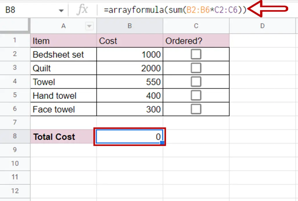
• Select the cell where the result is to be displayed
• Type the formula using cell references:

=ARRAYFORMULA(SUM(Cost*Ordered?))

• Press Enter

Step 2 – Check the result

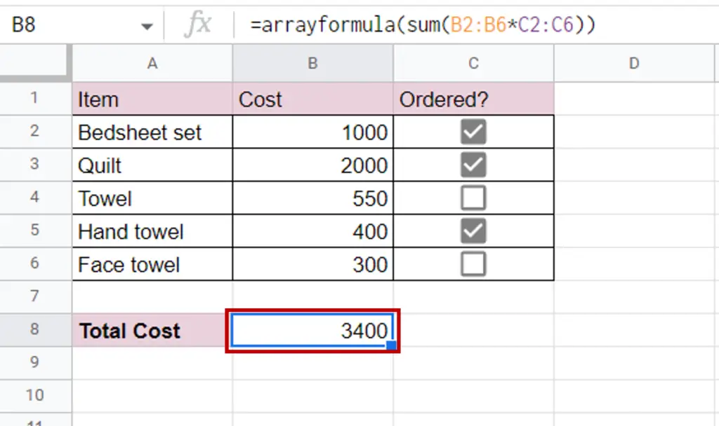
• Only those items whose checkbox is ticked will be included in the total cost

Option 2 – Use the keyboard shortcut

Step 1 – Create the formula

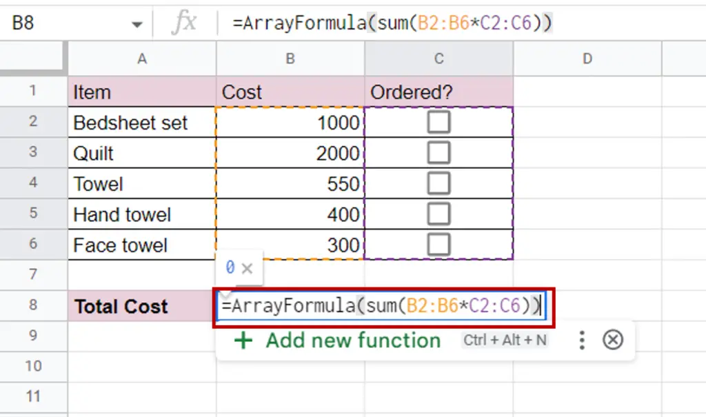
• Select the cell where the result is to be displayed
• Type the formula using cell references:

=SUM(Cost*Ordered?)

• Press Ctrl+Shift+Enter
• The ARRAYFORMULA() function is inserted into the formula
• Press Enter

Step 2 – Check the result

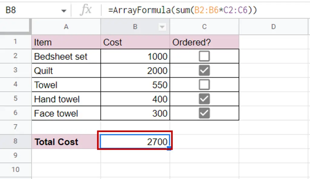
• Only those items whose checkbox is ticked will be included in the total cost