
How to remove total from a Pivot Table in Google Sheets
 By
SpreadCheaters
By
SpreadCheaters
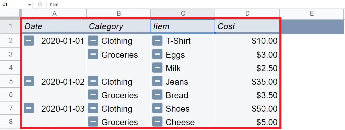
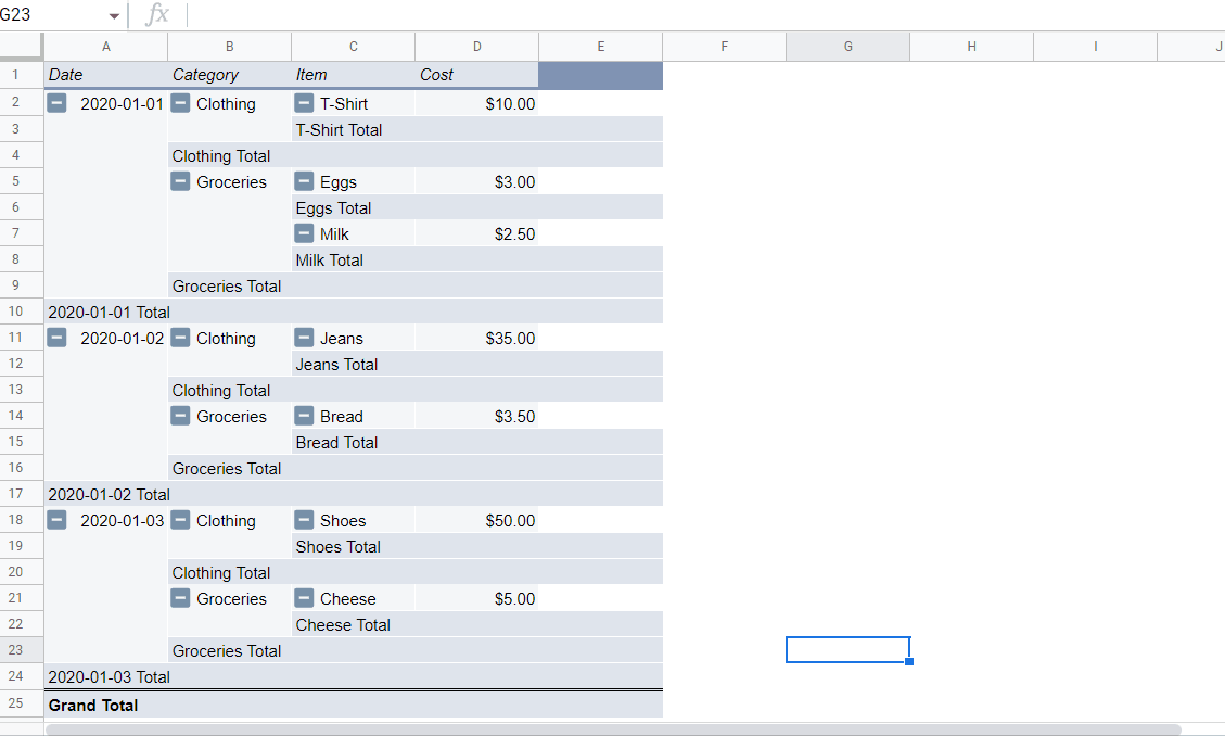
In this tutorial we will learn how to remove total from a pivot table in Google Sheets. In a pivot table, the total row provides a summary of the data in the pivot table. If you don’t need this information or would like to remove it, you can easily remove the total row from a pivot table. Here are the steps to remove the total row from a pivot table in Google Sheets.
Google Sheets is a free, web-based spreadsheet program offered by Google as part of its Google Drive service. It allows users to create and edit spreadsheets online, as well as share and collaborate on spreadsheets with others. Google Sheets offers a range of features, including cell formatting, data validation, conditional formatting, formula creation and calculation, and chart creation. It also includes a number of add-ons and tools, such as the pivot table, that can be used to analyze and summarize data.
Step 1 – Click anywhere on the pivot table
– Click anywhere on the pivot table or drag the cursor onto the pivot table.
– An Edit button will appear in the left bottom corner.
Step 2 – Click on the Edit button
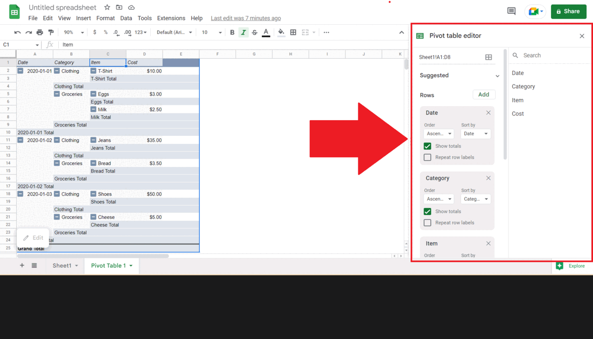
– Click on the Edit button, a window named “Pivot Table Editor” will appear on the left.
Step 3 – Unselect the “Show totals” option
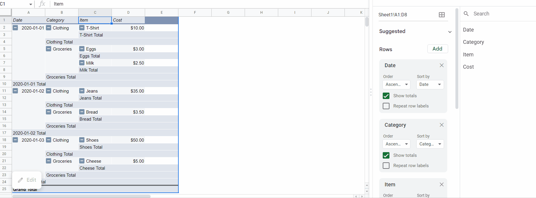
– Unselect the Show totals option in each header’s section.
Step 4 – Check if the Total has been Removed

– After unselecting show totals options, all the rows showing totals will be removed.


