
How to make a column stay in Google sheets
 By
SpreadCheaters
By
SpreadCheaters
You can watch a video tutorial here.

Freezing a pane is commonly used when scrolling through large amounts of data on a worksheet. When scrolling through a sheet that has a lot of data and either column headers or row names, it is difficult to keep track of the name of the row or column. Freezing either a row or column makes it possible to keep the row name or column header in place while you scroll through the rest of the data.
Step 1 – Navigate to the Freeze menu
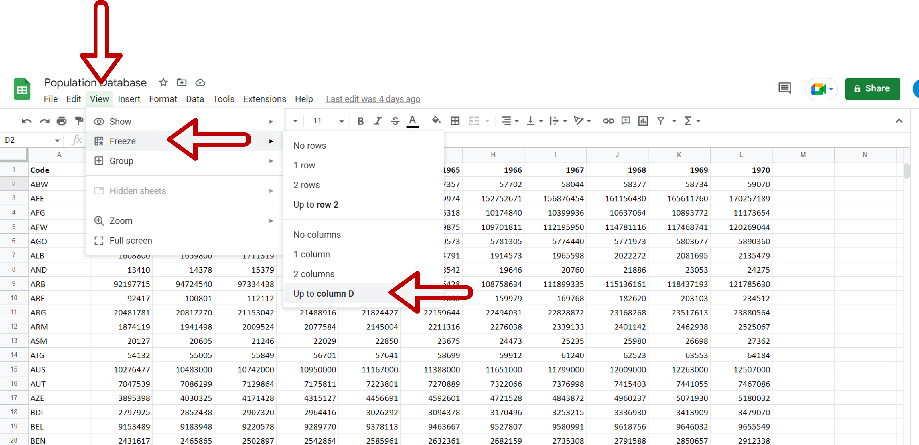
– Place the cursor in the column up to which you want the columns to stay
– Go to View > Freeze
– Select Up to column <your column number>
Step 2 – Check the result
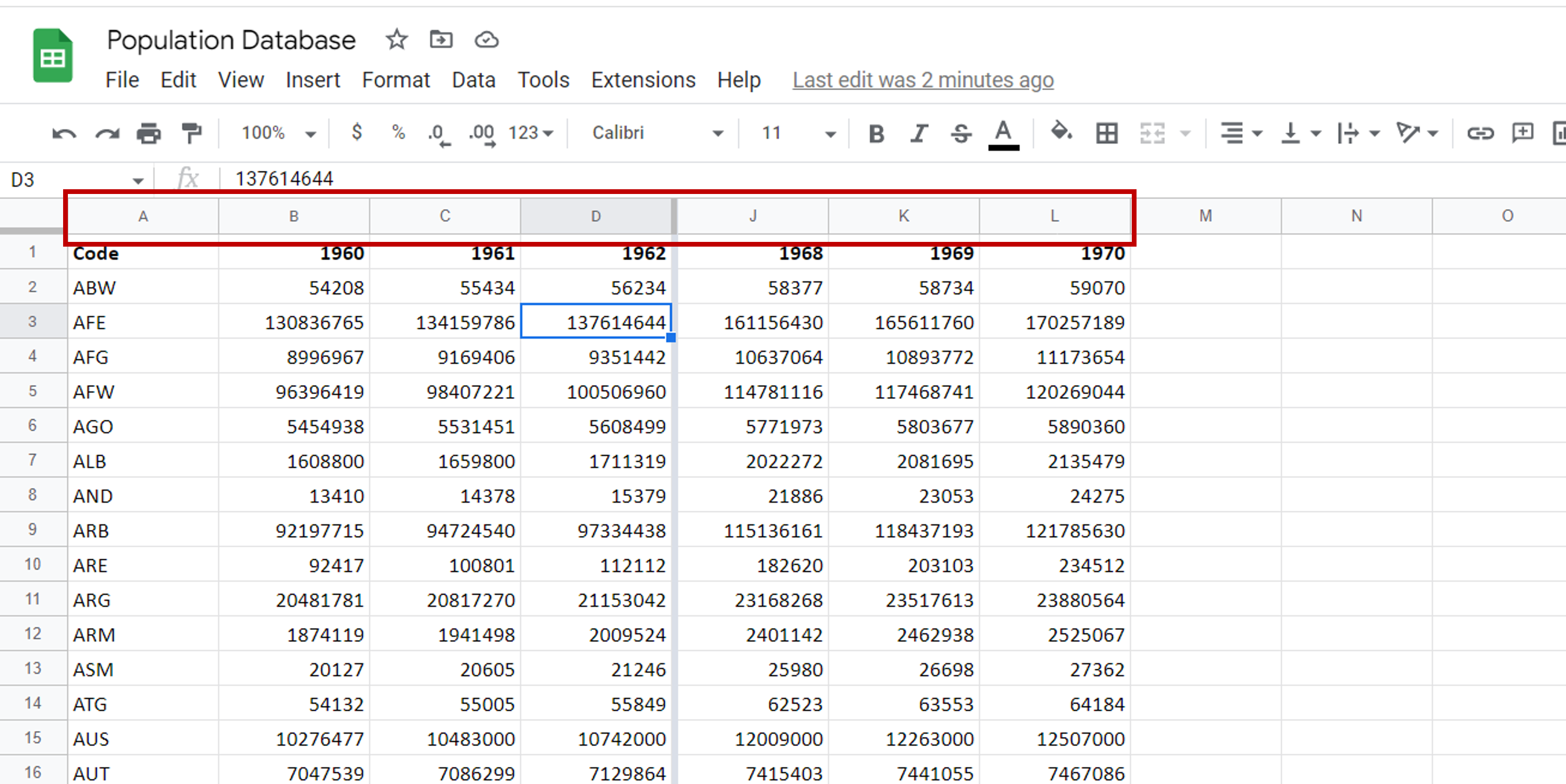
– Scroll to the right to check that the columns stay in place
Note: When freezing columns, only those to the left of the cursor can be locked. If the columns to the right have to be locked, you may need to rearrange the data.


