
How to label axis in Google Sheets
 By
SpreadCheaters
By
SpreadCheaters

Google Sheets offer a very interesting way to label axis. We can cater to this problem statement by using the chart customize option in google sheets. We can perform the below mentioned way to label axis in google sheets:
We’ll learn about this methodology step by step.
To do this yourself, please follow the steps described below;
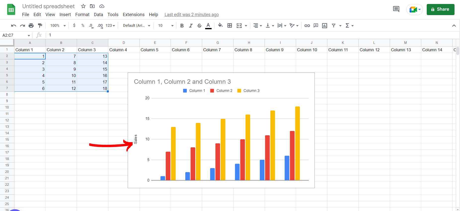
Step 1 – Google sheets tab with a list of random values and a chart
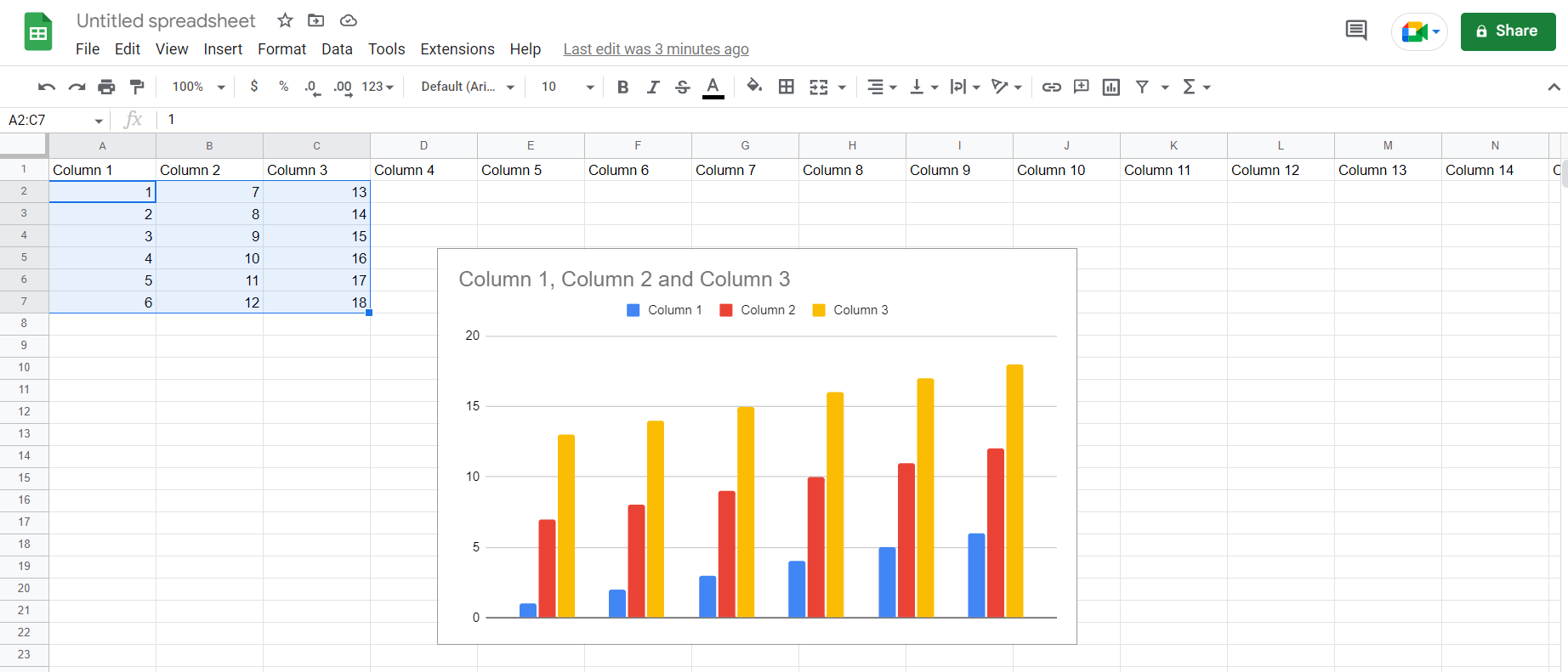
– Open the desired Google Sheets tab containing a chart as shown in the image above
Step 2 – Going to the edit chart option
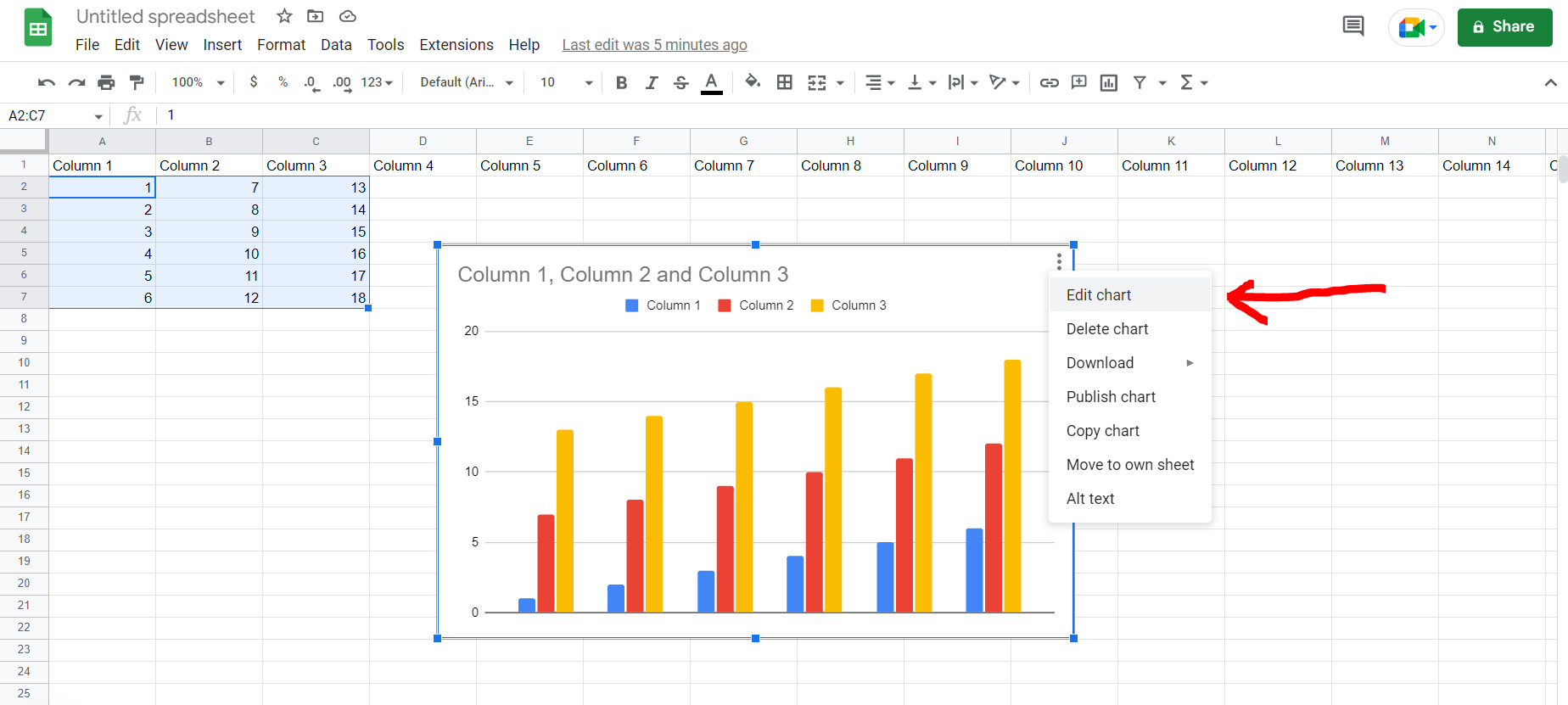
– Now click on the 3 vertical dots at the top right corner of the chart as shown in the image above, and then select the “Edit chart” option.
Step 3 – Customize option
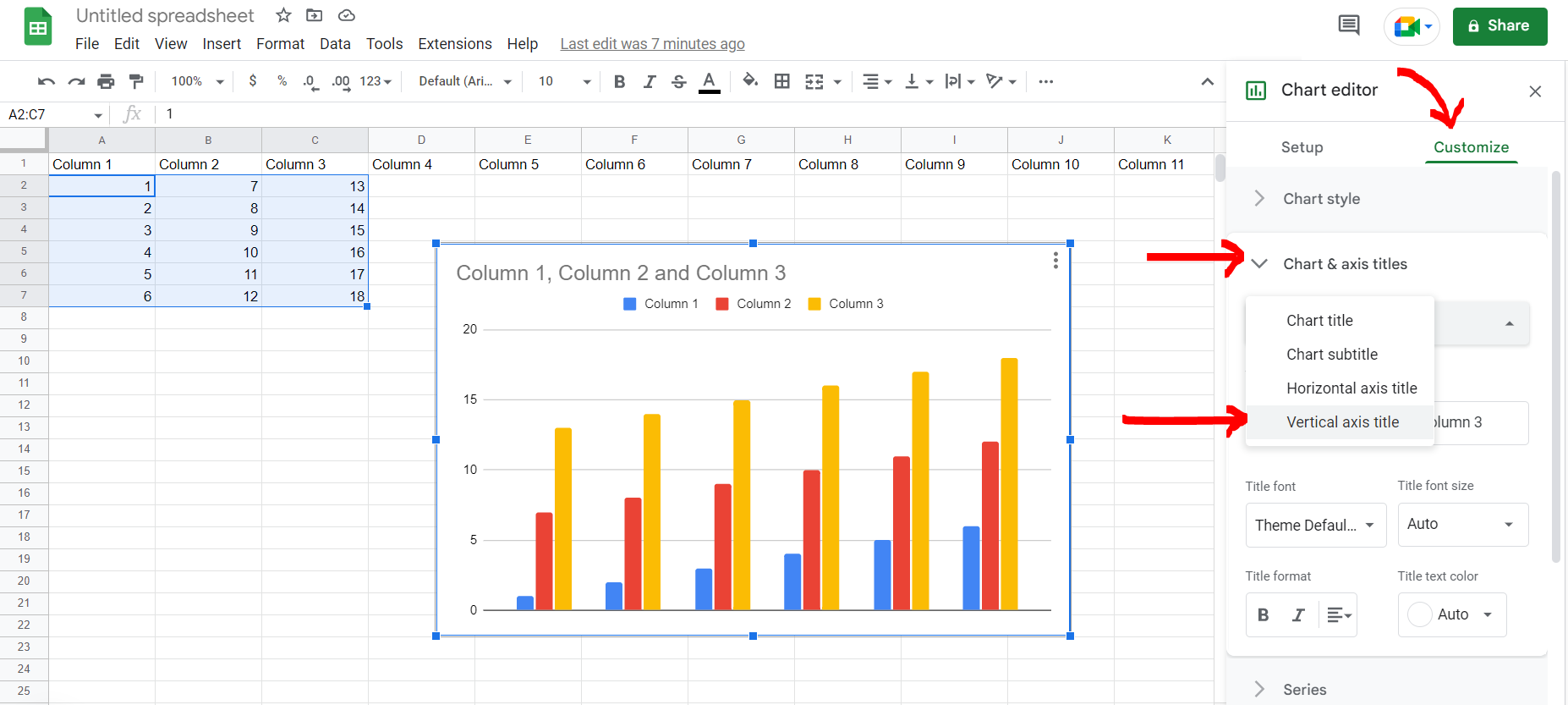
– Now a dialogue box will appear at the right of the screen. Click on the “Customize” option, then click on “Chart & sales titles”, then select the “Vertical axis title” from the drop down menu.
Step 4 – Typing the axis title
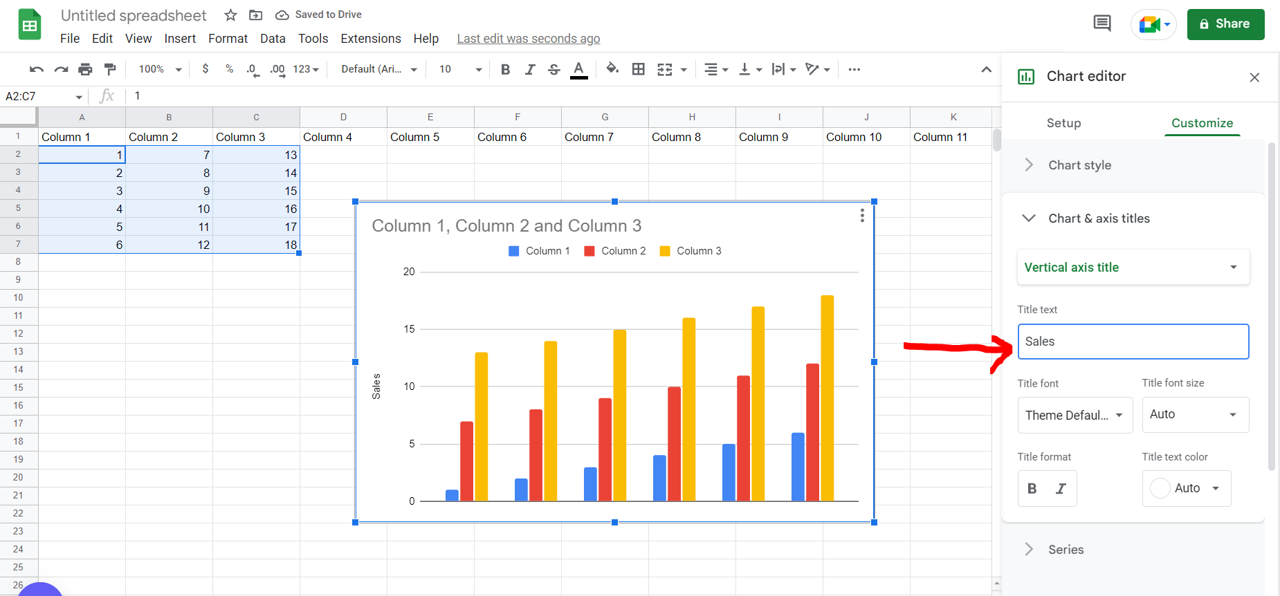
– Now under the “Title text” option type in the title of the labels on the axis, and then exit the Chart Editor side panel.
Step 5 – Axis labelled
– We can see that the axis has been labelled


