
How to keep a column fixed in Google Sheets
 By
SpreadCheaters
By
SpreadCheaters
You can watch a video tutorial here.
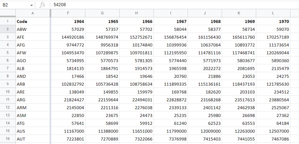
When scrolling through a sheet that has a lot of columns, it is difficult to keep track of the name of the rows. Also, if you have a worksheet that spans many columns and you want to compare data in two columns that are far apart from each other, you need a way to fix one column. Fixing a column makes it possible to keep the row name or a particular column locked in place while you scroll through the rest of the data.
Step 1 – Position the cursor

– Place the cursor in the column following the column you want to keep fixed
Step 2 – Navigate to the Freeze menu
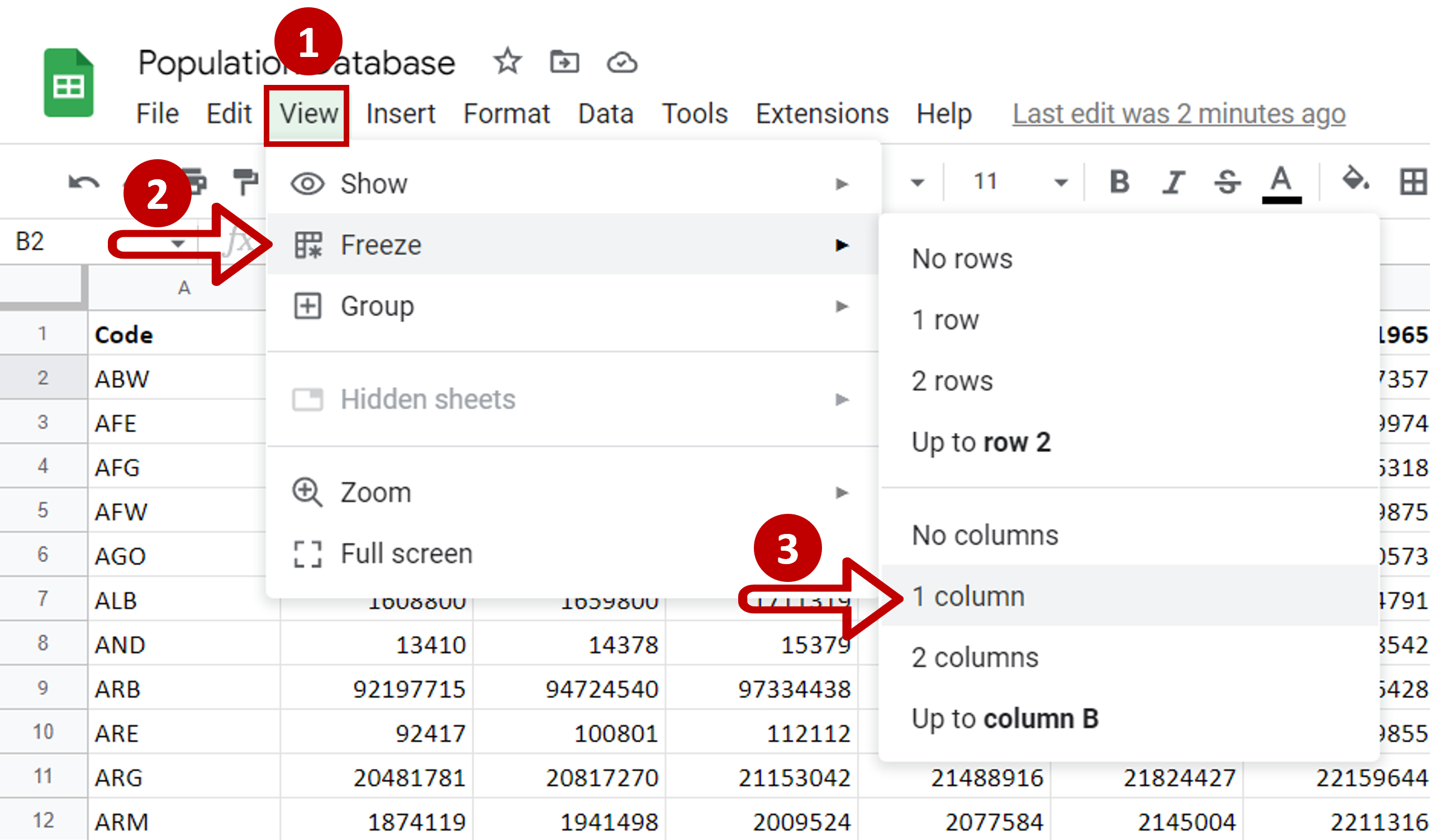
– Go to View > Freeze
– Select Up to column <your column number>
Step 3 – Check the result
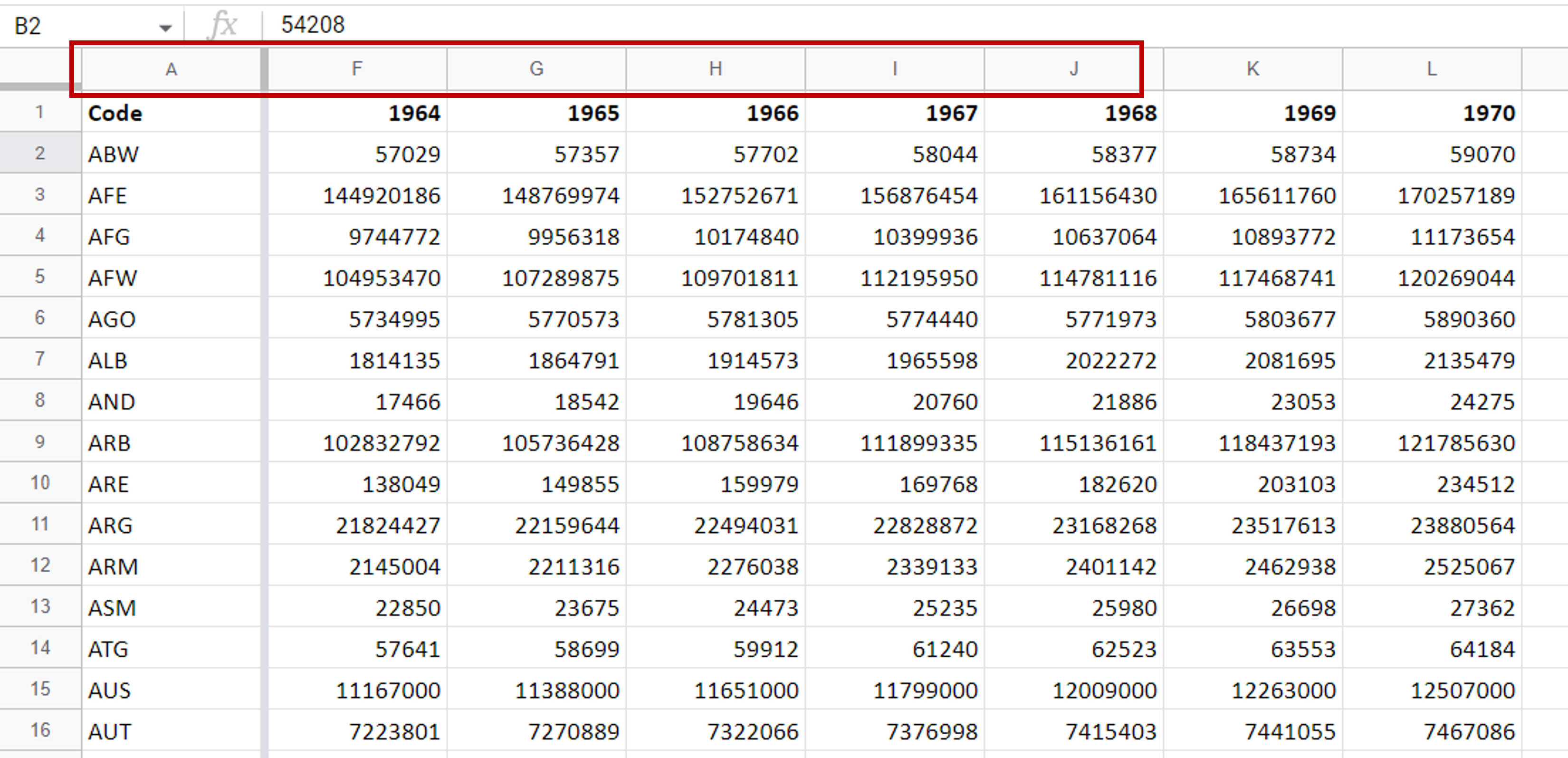
– Scroll to the right to check that the column stays in place
Note: When freezing columns, only those to the left of the cursor can be locked. If the columns to the right have to be locked, you may need to rearrange the data.


