How to group different rows in google sheets

Google sheet is a powerful tool for data calculation and data manipulations. In the Google sheet data is being stored in rows and columns. Google sheet is enriched with a lot of functions and tools. One such tool is the grouping of rows in Google Sheets. This tool is very useful for data scientists and when you are working with large datasets. This function groups the rows and an icon of (-) appears on the left, which is an icon of expansion. As we press it, only the first selected row stays visible, the rest of the rows will become invisible while keeping the data at its place. All the formulas will work accordingly. In this tutorial we’ll learn how to group rows in Google Sheets by using the following methods.

Method 1 – Use Right click option

By using this method we can use group rows, by right clicking on the serial number.

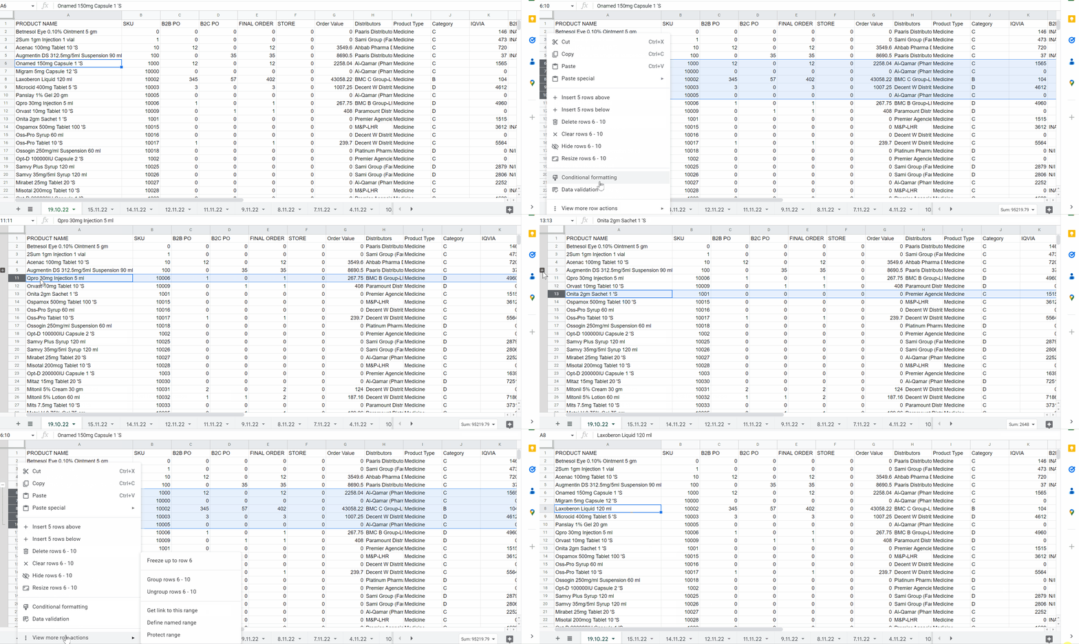
Step 1 – Group the rows by using context menu

• In the first place, select the rows that you wish to group.
• Right click on the serial number of the row.
• A menu will appear.
• Click on view more row actions.
• Click on Group rows.

Hence , we have successfully made a group of multiple rows and we can ungroup on the same pattern as shown in animation.

Method 2 – Use View tab

By using this method we can use group rows, a built-in function.

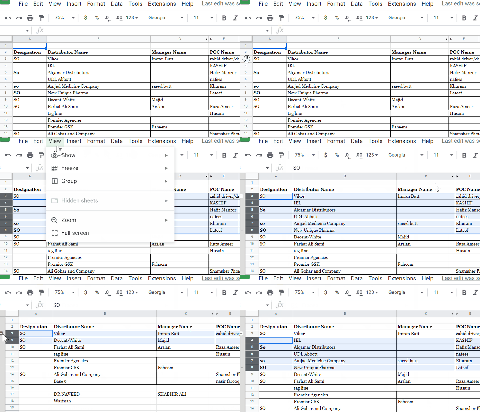
Step 1 – Select the rows and group 

• Select the rows.
• Go to View tab.
• Click on Group.
• A side menu will appear.
• Click on Group (serial number of rows).

It is clear that we can group rows in google sheets by two different methods.