How to get the sum of a column in Google Sheets

You can watch a video tutorial here.

Google Sheets is widely used for calculations due to the several arithmetic operators and functions that it has. You will frequently need to find the totals of columns of numbers. This can be easily done using the SUM function of Google Sheets. There are multiple ways in which the SUM function can be accessed.

Option 1 – Use the formula suggestion

Step 1 – Invoke the formula suggestion 

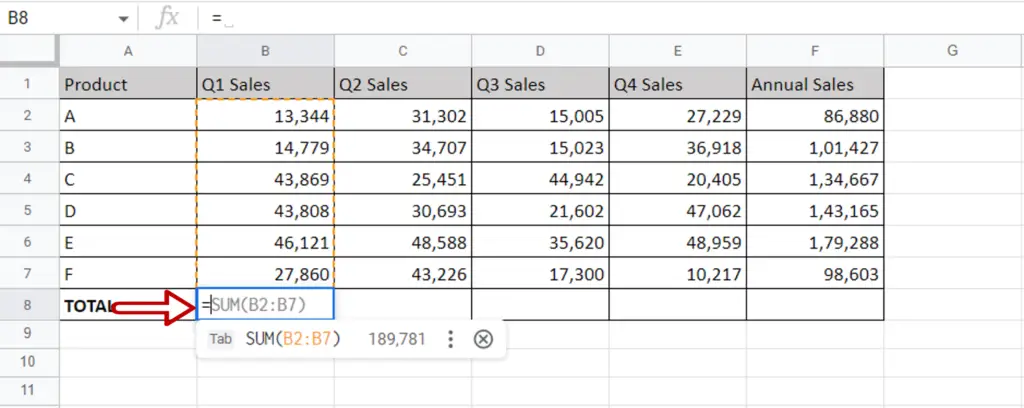
• In the destination cell, type an equal sign (=)
• The SUM function will be suggested

Note: If the formula suggestion does not appear, type the first letter of the function i.e. ‘S’. If it still does not appear, enable the feature by going to Tools > Autocomplete > Enable formula suggestions

Step 2 – Accept the formula suggestion

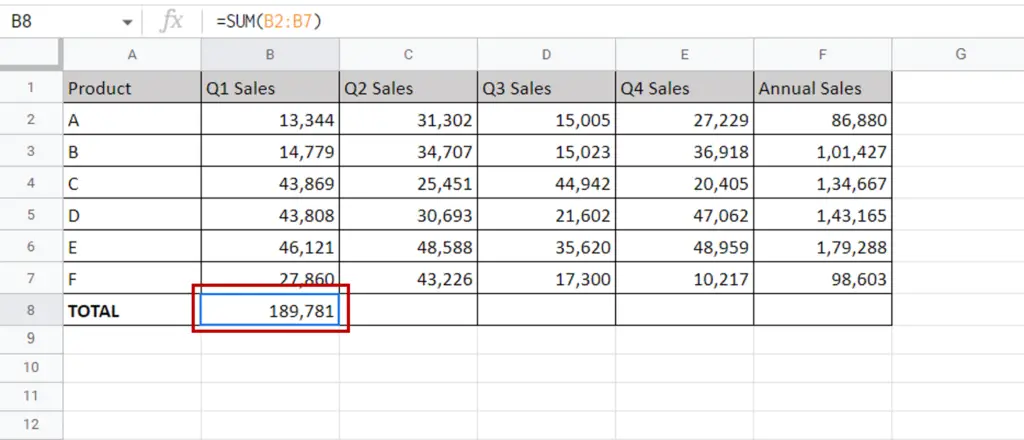
• Check that the range of cells is correct
• Press Enter
• The total of the numbers will be displayed

Option 2 – Use the Explore feature

Step 1 – Select the cells and open the Explore box

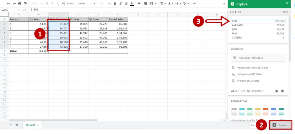
• Select the cells to be summed
• Click the Explore button at the bottom right of the sheet
• Select SUM from the box

Step 2 – Drag and drop the SUM function

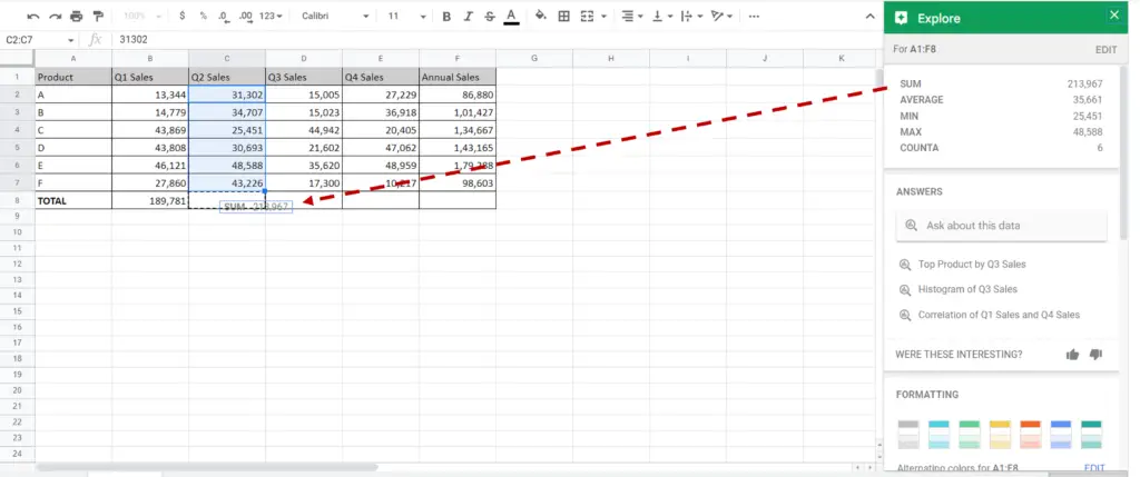
• Drag the SUM function and drop it into the destination cell

Option 3 – Use the menu option

Step 1 – Insert the SUM function

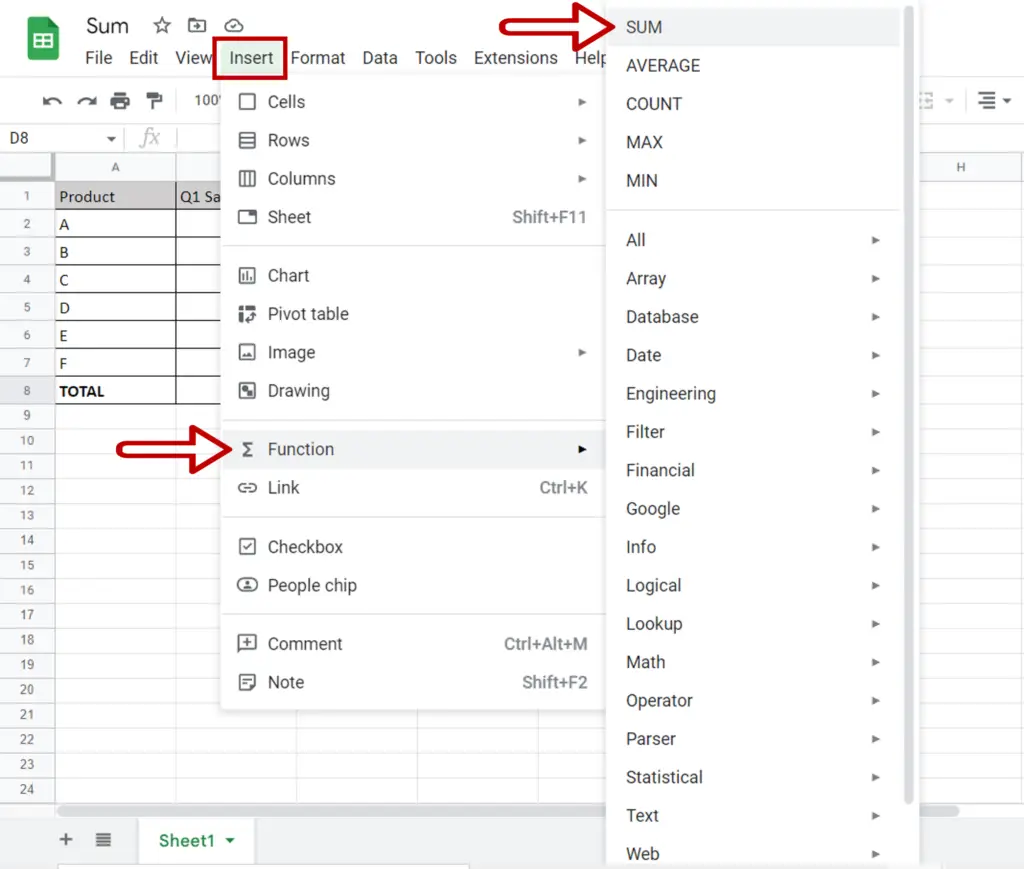
• Select the destination cell of the total
• Go to Insert > Function 
• Click SUM

Step 2 – Select the range

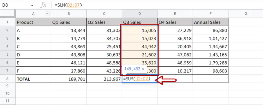
• The SUM function will be inserted into the destination cell, ready to accept the range
• Select the range of cells to be summed
• Press Enter

Option 4 – Type the SUM() function

Step 1 – Enter the formula

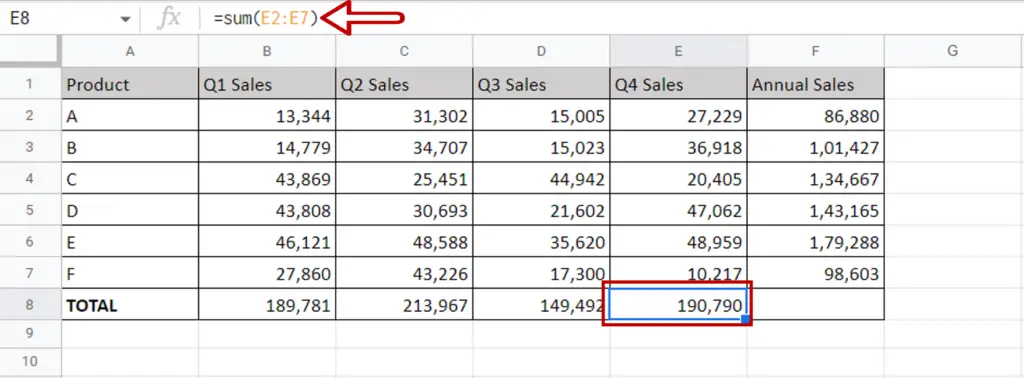
• Select the destination cell of the total
• Type the formula using the range:

=SUM(Range of Q4 Sales)

• Press Enter