
How to Freeze Panes (multiple rows & columns) in Google Sheets
 By
SpreadCheaters
By
SpreadCheaters
Google Sheets offer some very interesting features to handle large data sets. These features are very handy when we want to navigate through the data in a Google Sheet with a big data set, i.e. rows and columns of the order of 100s to 1000s. In this tutorial we’ll learn how to freeze panes (multiple rows and columns) in Google Sheets by following these steps.
Step 1 – Locate the View tab
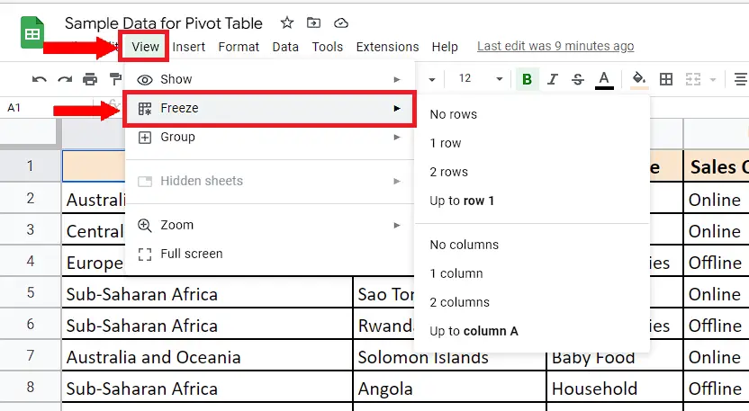
– Open the desired Google Sheet in which you want to freeze panes.
– Navigate to “View Tab” from the list of main tabs available at the top row as shown above.
Step 2 – Select the appropriate cell
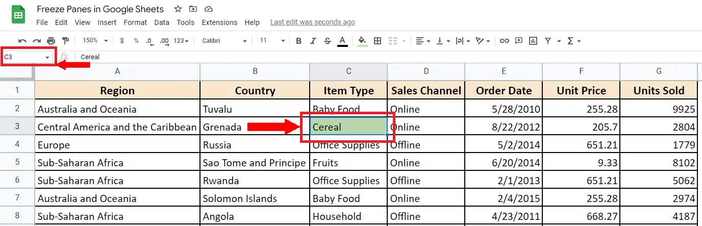
– Now comes the tricky part, you will have to select a specific cell before activating this feature. The location of this specific cell will depend upon the following two things;
a) Number of rows you want to freeze.
b) Number of columns you want to freeze.
Let’s just say that you want to freeze the first three (3) rows and first three (3) columns i.e. up to column C, then you will have to select the cell which lies at the intersection of third (3rd) row and third column i.e. column C. So following the above mentioned logic, the location of the cell comes out to be 3rd row in Column C i.e. C3. The key cell is highlighted with green colour in the picture below to explain the procedure of cell selection.
Step 3 – Freeze Selected Rows up to row 3
– After selecting the cell as per the instruction given above, you are all set to activate the feature to freeze the first three (3) rows & first three (3) columns. All you have to do is to go to “View Tab” again and in that tab locate the “Freeze” option.
– Unlike Excel, where we can freeze the pane by just one click, we’ll have to freeze the desired rows and columns one by one. So, choose the option Up to row 3 in the Freeze category.
– This will freeze the first 3 rows as shown above.
Step 4 – Freeze Selected Columns up to column C

– As described in the earlier step, unlike Excel, where we can freeze the pane by just one click, we’ll have to freeze the desired rows and columns one by one. We have frozen the rows in the last step, so now choose the option up to column C in the Freeze category.
– This will freeze the first 3 columns and finally we’ll have our pane of 3 rows and 3 columns frozen as well as shown above.


