How to freeze a row in google sheets

You can watch a video tutorial here.

Any number of rows and/or columns in a Google sheet can be frozen so that they always stay in the same place while the rest of the sheet is moved around.

There are three possible solutions:

Solution 1 – Using the main menu

Step 1 – Click on the View > Freeze menu option in the GSheet and select the number of rows or columns that you would like to “freeze”

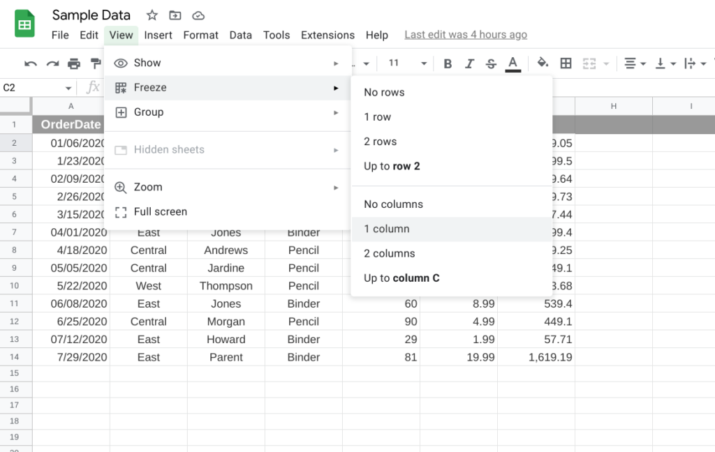
• Click on the View > Freeze menu option in the GSheet and select the number of rows or columns that you would like to “freeze”

Solution 2 – Hovering over the row/column boundary

Step 1 – By hovering over the right hand edge of the column containing the row numbers, or the bottom edge of the row containing the column letters a little hand cursor appears which can be used to drag the required number of rows or columns.

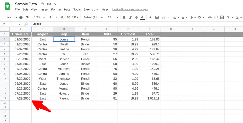
• By hovering over the right hand edge of the column containing the row numbers, or the bottom edge of the row containing the column letters a little hand cursor appears which can be used to drag the required number of rows or columns.

Solution 3 – Using the row/column context (right-click) menu

Step 1 – Select a full row or column that you want to freeze up to by clicking on the appropriate number or letter

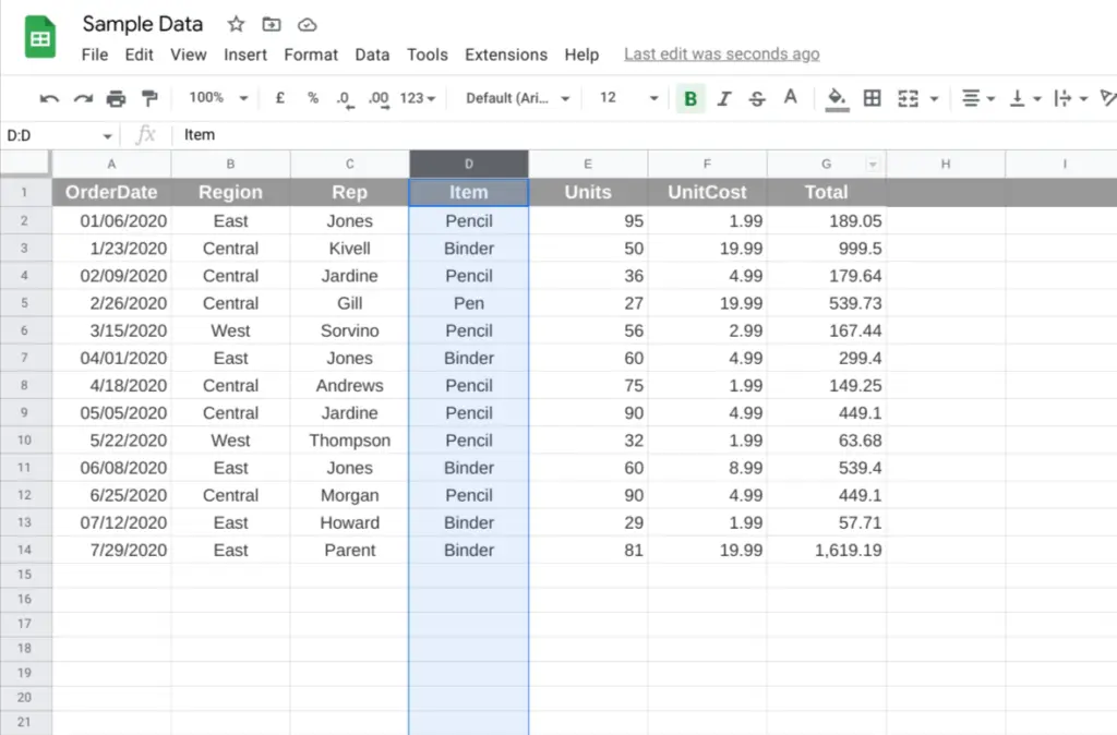
• Select a full row or column that you want to freeze up to by clicking on the appropriate number or letter

Step 2 – Use the mouse right-click button to open the context menu, and click on, in this case, “View more column actions > Freeze up to column D”

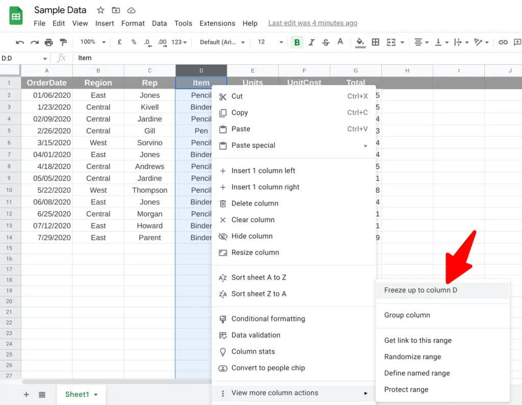
• Use the mouse right-click button to open the context menu, and click on, in this case, “View more column actions > Freeze up to column D”