
How to freeze a cell in Google Sheets
 By
SpreadCheaters
By
SpreadCheaters

Google sheets offer a very interesting way to freeze a cell. We can perform the below mentioned way to use freeze cell in google sheets:
We’ll learn about this methodology step by step.
To do this yourself, please follow the steps described below;
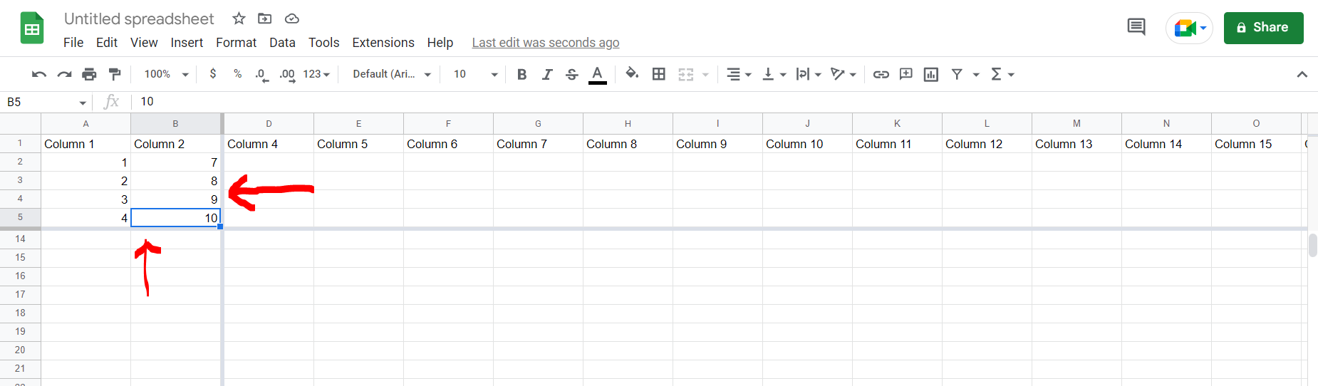
Step 1 – Google sheet with multiple columns and rows
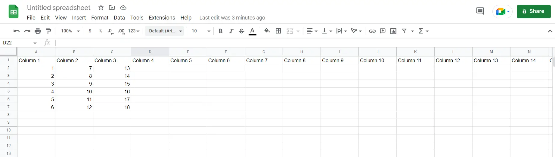
– Open the desired Google Sheet which contains multiple columns and rows as we have in the image above
Step 2 – Making the required cell active
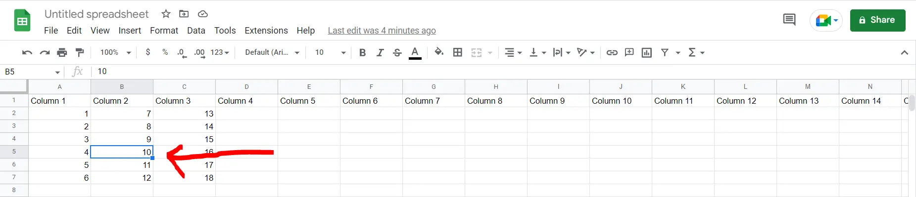
– Now select any of the required cells which need to be frozen.
Step 3 – Freezing the column
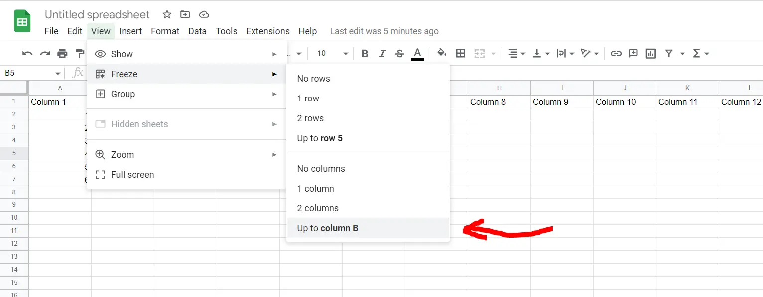
– Go to the View option, then click on “Freeze”, then click on “Up to column X”(Where X is the column of the active cell). This will freeze the column where we have our cell active (in our case column B)
Step 4 – Freezing the row
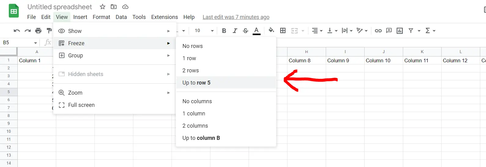
– Go to the View option, then click on “Freeze”, then click on “Up to row X”(Where X is the row of the active cell). This will freeze the row where we have our cell active (in our case row 5)
Step 5 – Cell frozen
– We can now see that after scrolling towards the right or to the bottom, our selected cell remains stationary, hence we have frozen the cell.


