
How to do bullet points in Google Sheets
 By
SpreadCheaters
By
SpreadCheaters
You can watch a video tutorial here.
Bullet points are an effective tool to communicate information concisely. When you have a list of instructions, it is better to make them into a series of bullet points so that each step is clear and the scope for misunderstanding on the part of the user is reduced. Google Sheets does not provide a formatting option to add bullet points to text, but there are some workarounds:
- Using the keyboard shortcut
- Using the CHAR() function: this converts a Unicode number into the corresponding character
- Syntax: CHAR(Unicode number)
- Unicode number: the Unicode standard has a unique number for every character (numbers, letters, punctuation, symbols, etc.). This number is common across all platforms and software languages. The Unicode number used in Google Sheets will display the same character when used in Excel.
- Syntax: CHAR(Unicode number)
- Creating a custom format
Option 1 – Use the keyboard shortcut
Step 1 – Add the bullet point
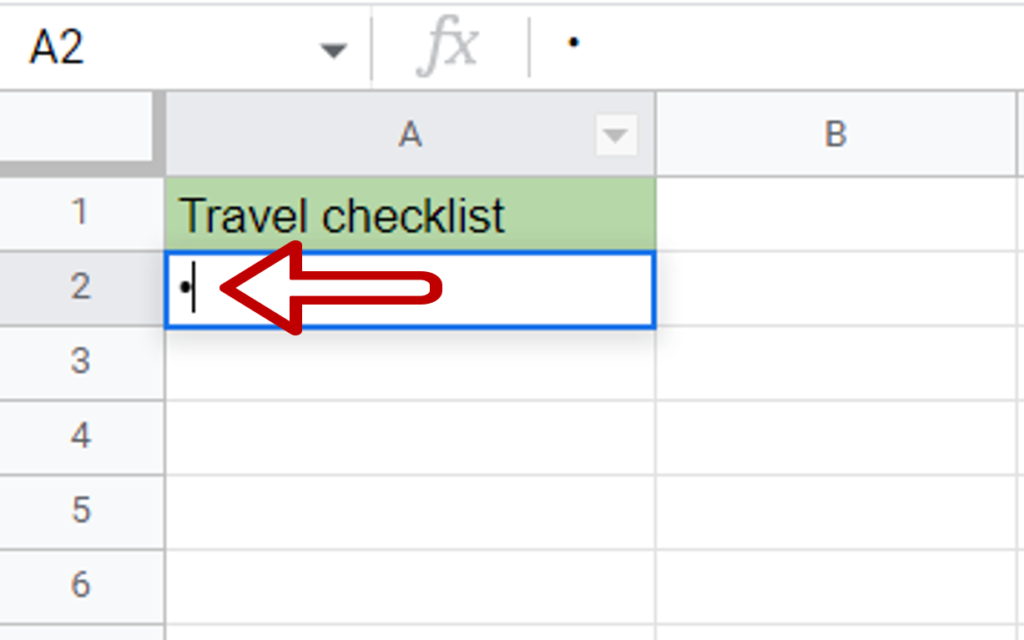
- Select the cell where the bullet point is to be added
- Press F2 to edit the cell
- Press ALT+7 to add the bullet point
Step 2 – Type the text
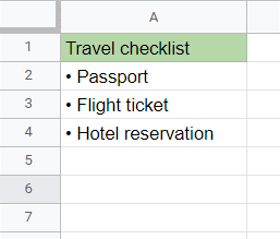
- Type the text after the bullet point
- Repeat this for every item in the list
Option 2 – Use the CHAR() function
Step 1 – Join the CHAR() function to the text
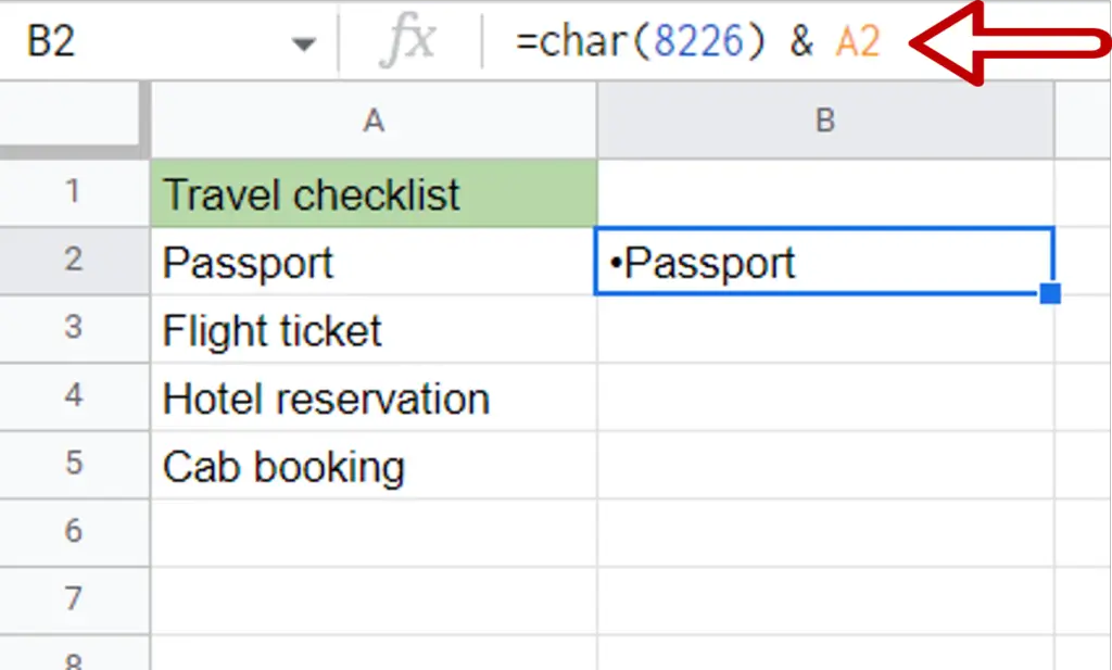
- Select the first cell of the column next to the list that is to be bulleted
- Type the formula using the cell references:
=CHAR(8826) & <text>
- Press Enter
- The list is displayed with bullet points
Note: 8826 is the Unicode number for one type of checkmark. You can use any of the many resources on the internet to find Unicode numbers for other characters.
Step 2 – Copy the formula
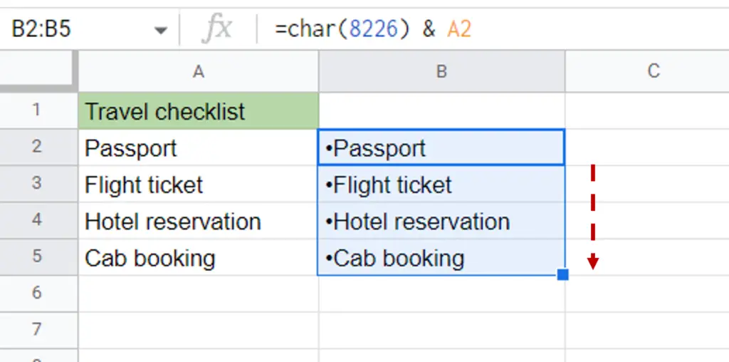
- Using the fill handle from the first cell, drag the formula to the remaining cells
OR
- Select the cell with the formula and press Ctrl+C or choose Copy from the context menu (right-click)
- Select the rest of the cells in the column and press Ctrl+V or choose Paste from the context menu (right-click)
Option 3 – Create a custom format
Step 1 – Select the list
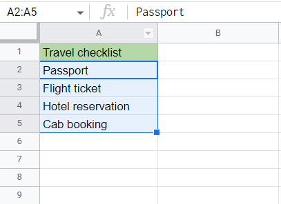
- Select the range of cells that are to be bulleted
Step 2 – Open the Custom number formats box
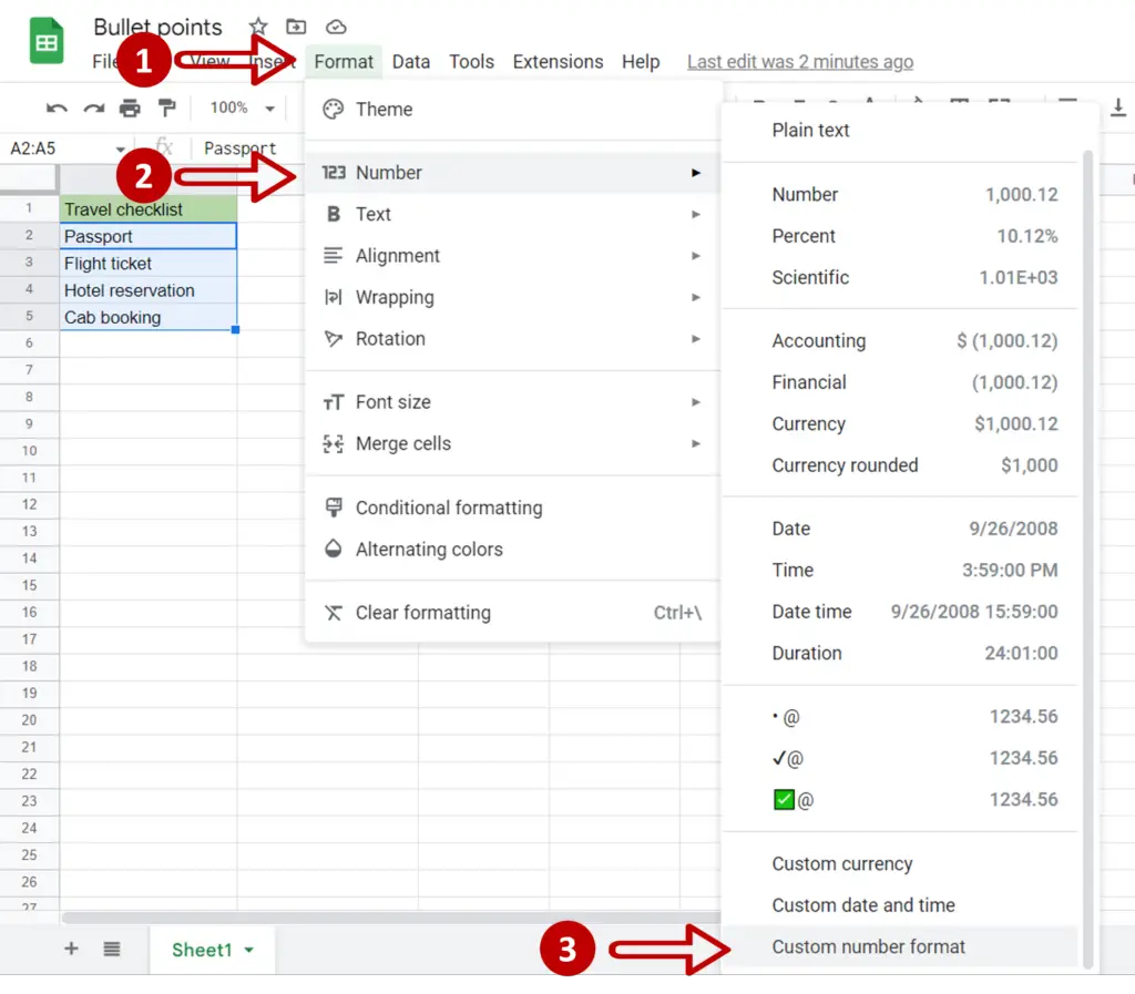
- Go to Format > Number > Custom number format
Step 3 – Define the format
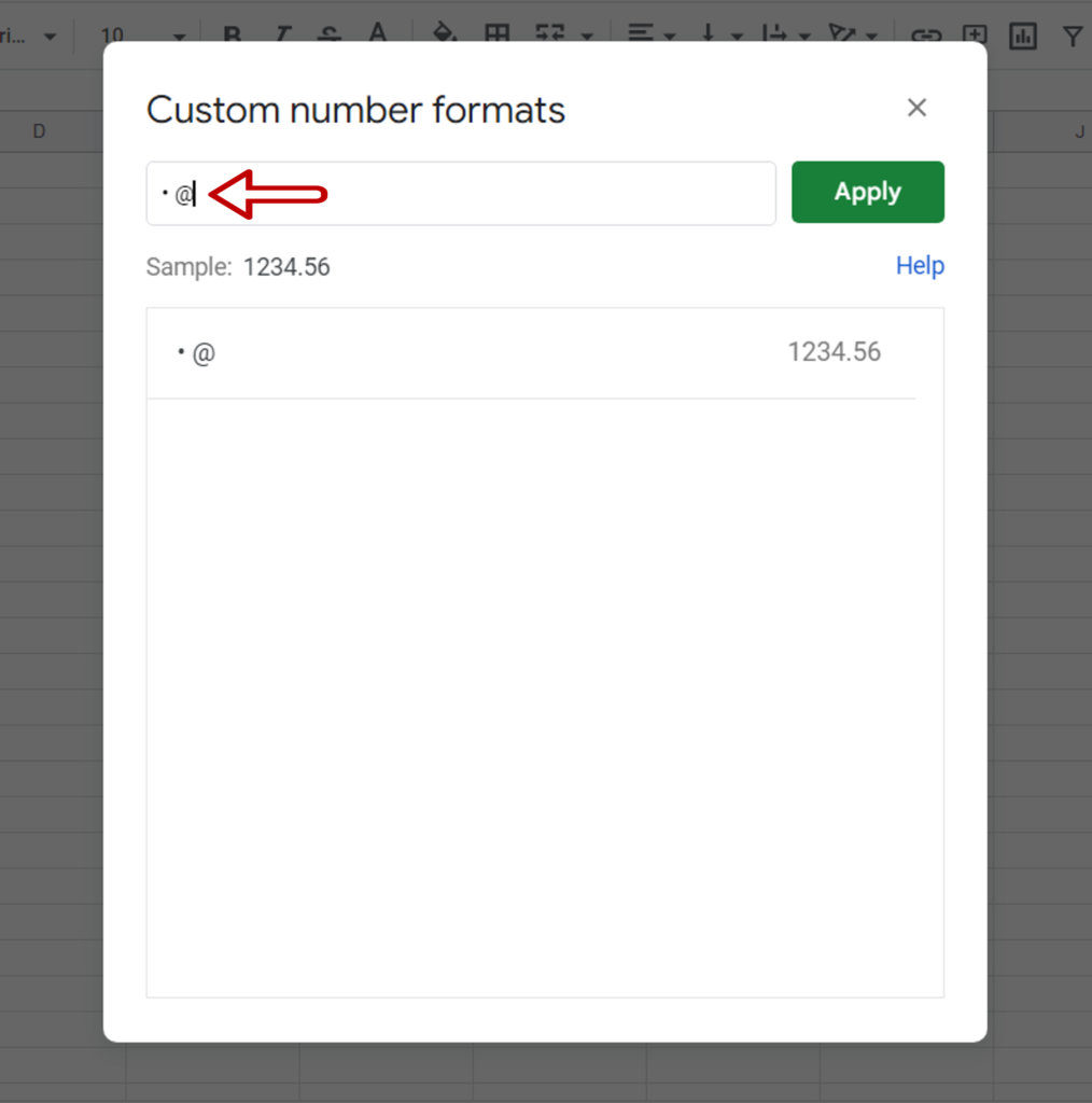
- In the editable box press Alt+7 followed by ‘@’
- Click Apply
Step 4 – Check the result
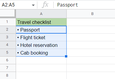
- Bullet points will be added to the list
Note: This method can be used to format blank cells as well. When text is typed in the cells formatted with the custom bullet format, bullet points will be added automatically


