
How to create a filter in Google Sheets
 By
SpreadCheaters
By
SpreadCheaters
You can watch a video tutorial here.
In Google Sheets, filters are a popular way of creating a subset of the data to analyze it or to perform data cleaning operations. As long as the data is organized in columns, the filter can be applied to any column, even if the column does not have a header. To filter data you need to specify one or more criteria and only the rows that match those criteria are displayed. The rows that do not match the results are hidden. When you remove the criteria, all the rows are displayed again. In Google Sheets, you can create and save a filter under a name. This can be done for filters that are frequently applied to the data.
Step 1 – Open the filter definition view
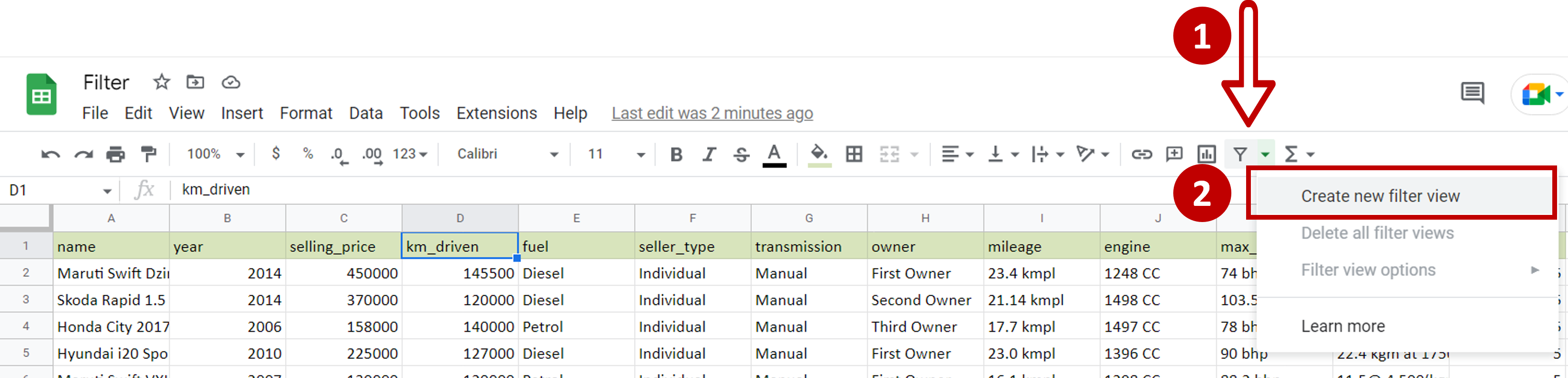
– On the ribbon click the Filter views button
– Click Create new filter view
Step 2 – Open the filter box
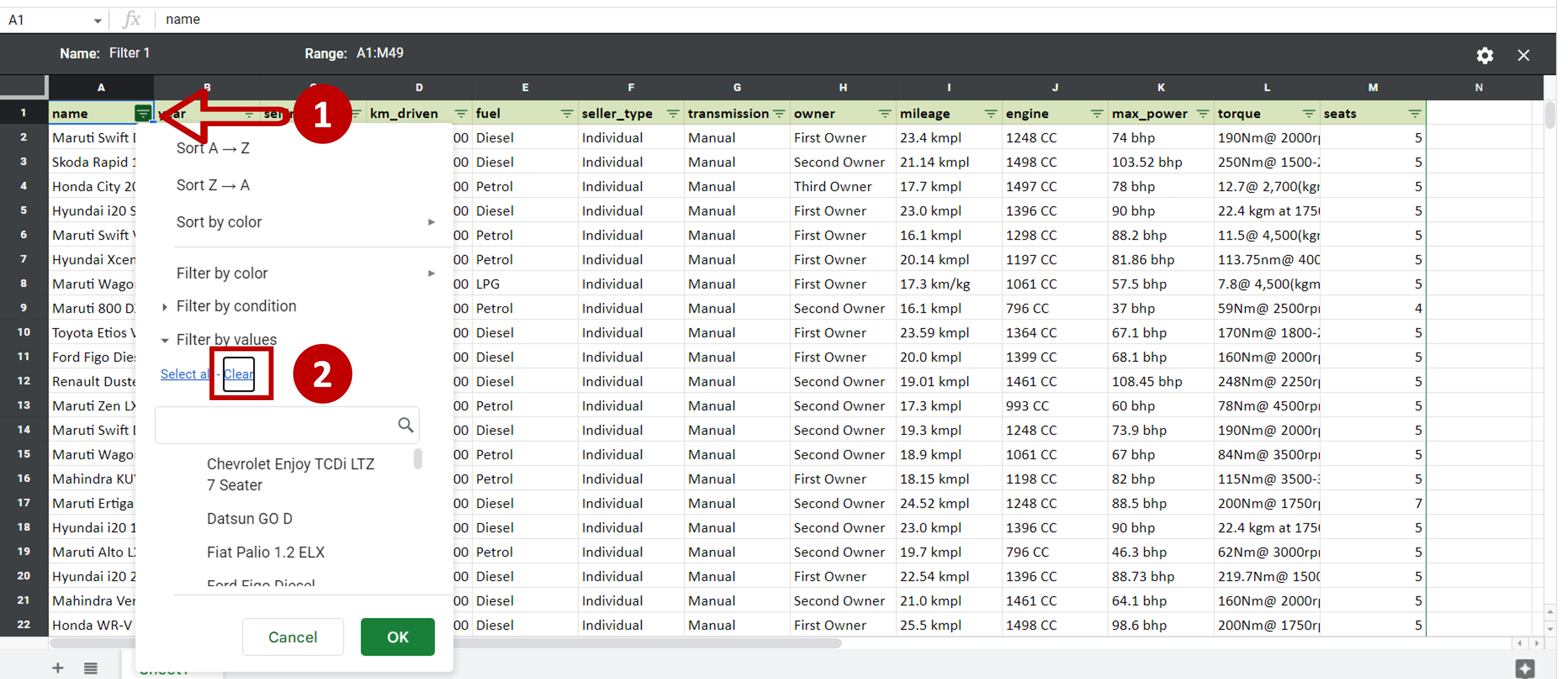
– Click the filter button in the ‘name’ column
– In the search box type click Clear
Step 3 – Set the filter condition
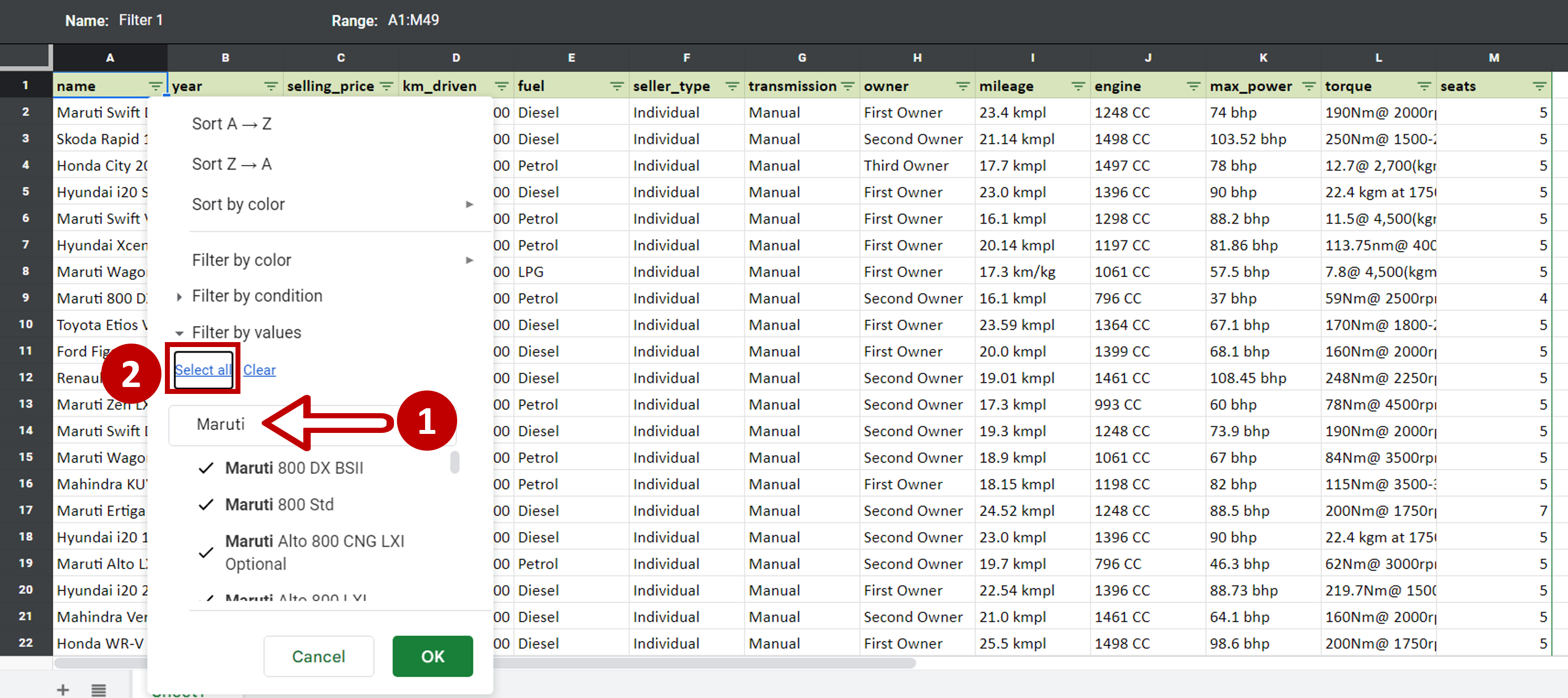
– In the search box type ‘Maruti’
– Click Select all
– Click OK
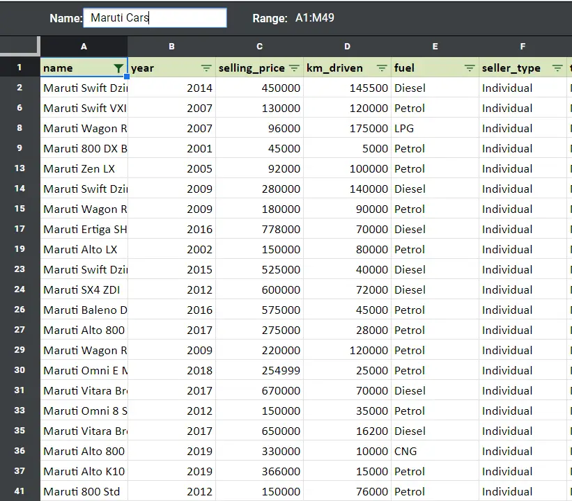
Step 4 – Check the result and name the filter
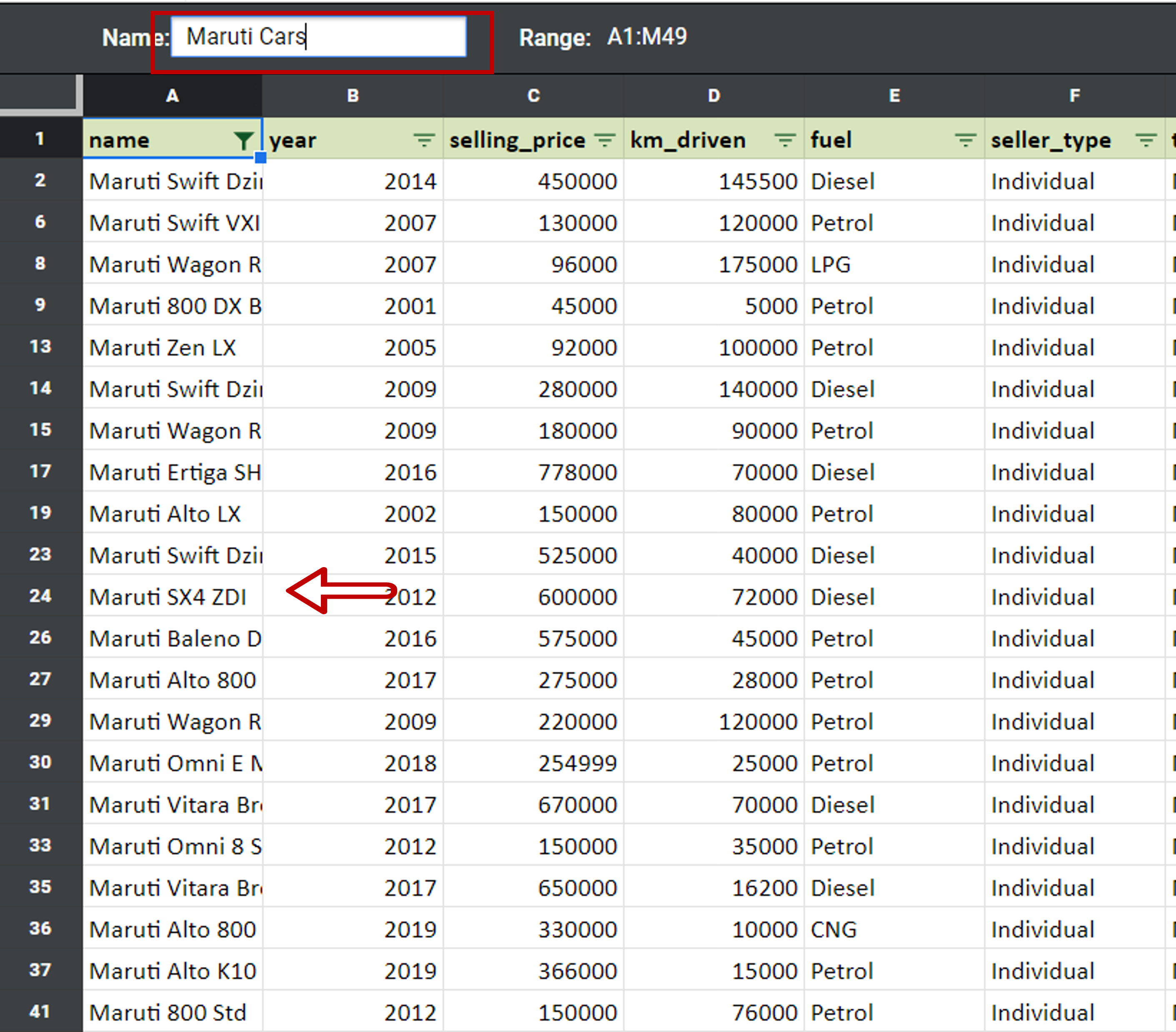
– Only those rows that have ‘Maruti’ in the ‘name’ column are displayed
– A filter symbol appears on the in-column filter in the ‘name’ column to indicate that a filter has been applied
– In the Name field, type ‘Maruti Cars’
Step 5 – Close the filter
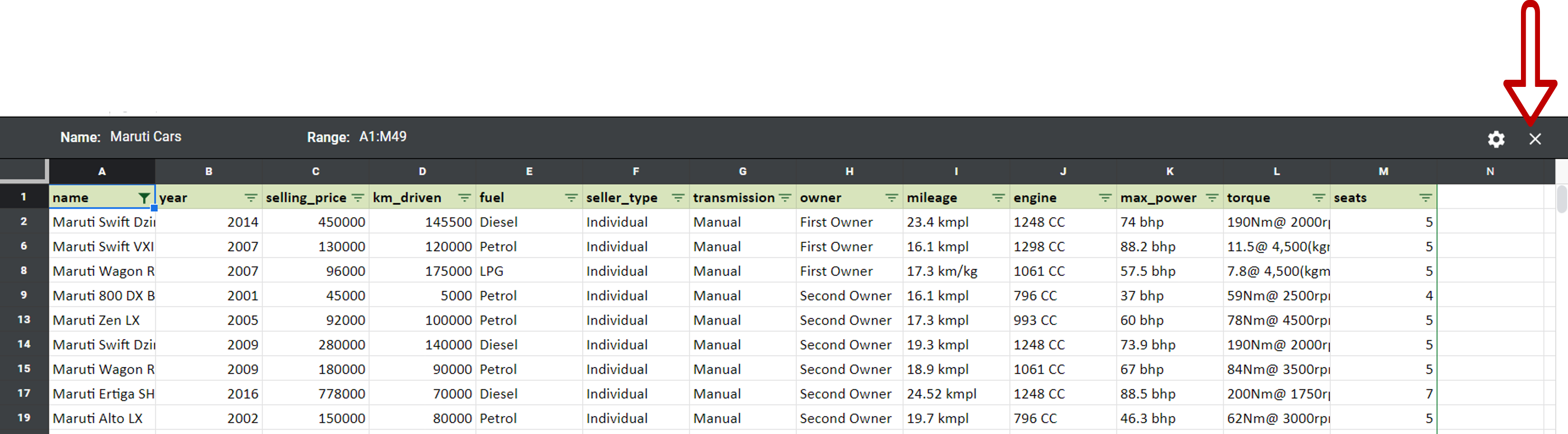
– Click on the cross to close the filter
Step 6 – Check that the filter has been created
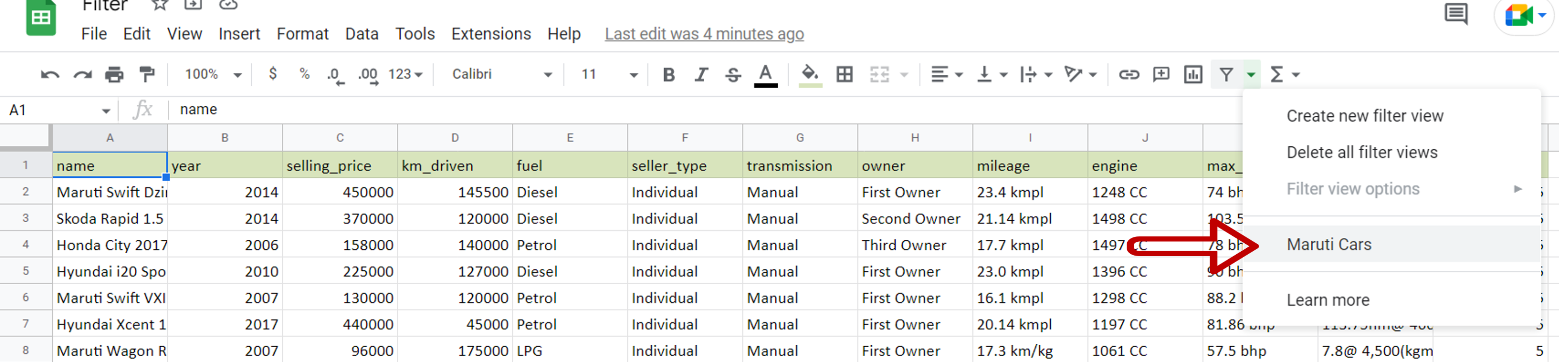
– On the ribbon click the Filter views button
– Check that the ‘Maruti Cars’ filter is listed


