
How to count colored cells in Google Sheets
 By
SpreadCheaters
By
SpreadCheaters
You can watch a video tutorial here.
Using conditional formatting, it is possible to highlight cells based on their value. You can also choose to highlight cells by changing the background color of the cell. If you then need to count the colored cells, you can do so using the SUBTOTAL() function and a filter.
1. SUBTOTAL() function: this returns the subtotal for a column using a specified aggregation function
a. Syntax: SUBTOTAL(function_code, ranges)
i. function_code: this is a number that corresponds to an aggregation function e.g. 1 is AVERAGE, 2 is COUNT, etc.
ii. ranges: the range of the cells on which the function is to be applied
Step 1 – Create the SUBTOTAL() function
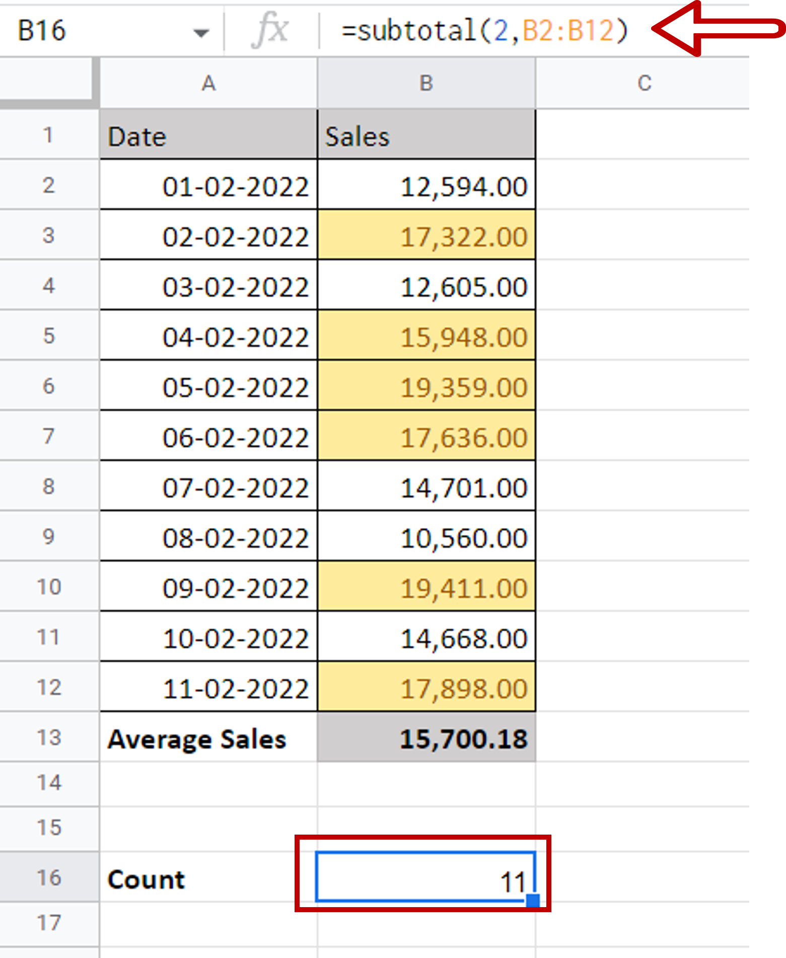
– Select the cell where the result is to appear
– The cell should be below the data otherwise it will be lost when the rows are filtered
– Type the formula using cell references:
=SUBTOTAL(2, <range of the ‘Sales’ column>)
Note: 2 represents the COUNT function
Step 2 – Turn on the in-column filters
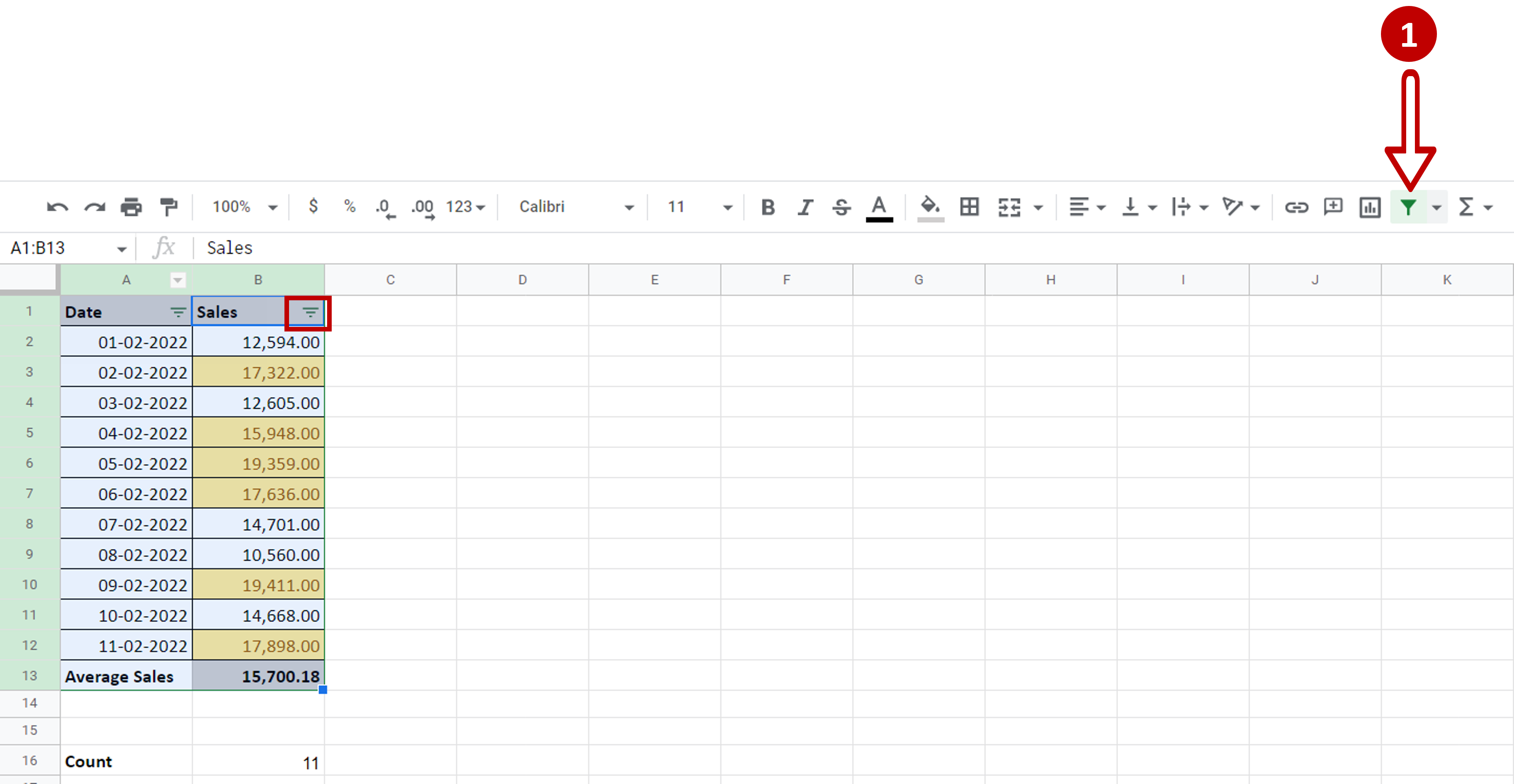
– Click the Filter button on the ribbon
Step 3 – Choose the filter
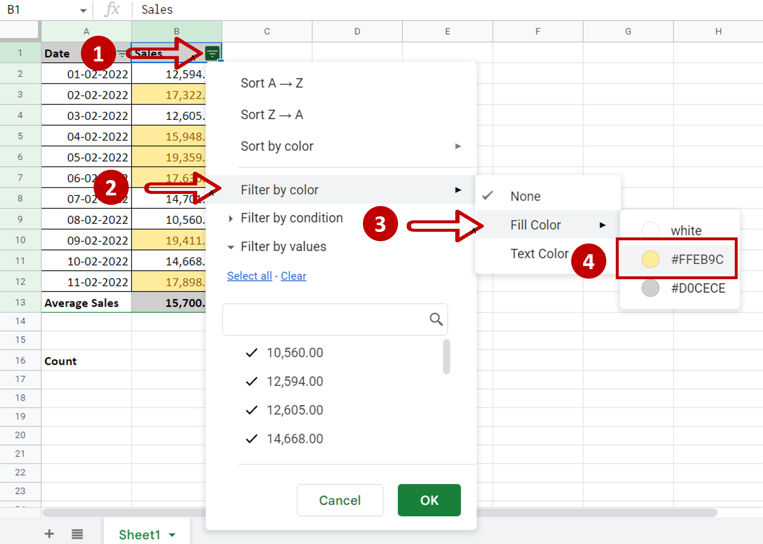
– Expand the filter drop-down menu by clicking on it
– Choose Filter by color > Fill color
– Choose the color of the highlighted cells
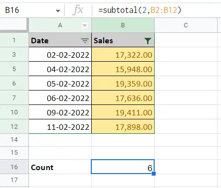
Step 4 – Check the count
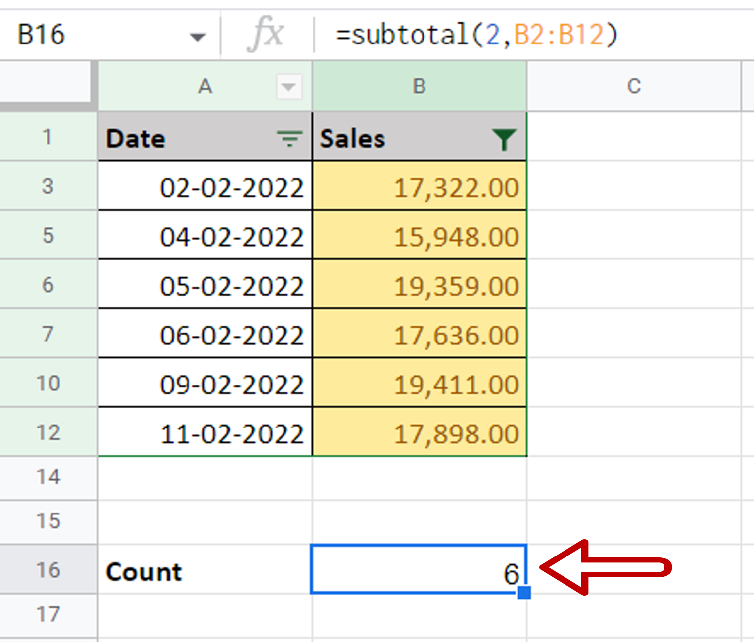
– The SUBTOTAL() function will display the count of the filtered i.e. the colored cells


