
How to compare two columns in Google Sheets
 By
SpreadCheaters
By
SpreadCheaters
You can watch a video tutorial here.
Google Sheets is a cloud-based spreadsheet application developed by Google. Users can create and edit spreadsheets online, and can also collaborate in real-time with other users while creating and editing spreadsheets. Some of its key features and functions include: editing and sharing spreadsheets, sorting and filtering data, formula creation and execution, data visualization, and many more.
In this step-by-step guide, you will learn to compare two columns for differences and similarities. Here we have a data set of two restaurants above which have some common and uncommon items in their menus.
Method 1: Compare Two Columns for Row Matches
We’ll write a formula to compare two columns for a row. If they have something in common it will be marked as ‘TRUE’ or else it will be marked as ‘FALSE’. Follow the below given steps:
Step 1 – Add an extra column

- Add an extra column in which the calculated comparison will be displayed.
- In this example, we named it ‘Comparison’
Step 2 – Enter the formula
- Select the top cell of the column. In our case, we are using ‘C2’.
- We will use the following formula ‘Syntax =First cell =Second cell’. In our case, we are comparing cells in the same row i.e. A2 and B2 so, the formula will be:
=A2=B2
- Type the formula and press the ‘Enter’ button. You will get the result whether it’s true or false.
Step 3 – Apply the formula to whole column
- Now, drag the (■) symbol.
- Doing this will copy the formula to all the cells of the Comparison column.
Step 4 – Get the comparison of both menus
- The same menu items will be marked as ‘TRUE’.
- The uncommon/different items will be marked as ‘FALSE’.
Method 2: Compare Two Columns to return a Predefined Value
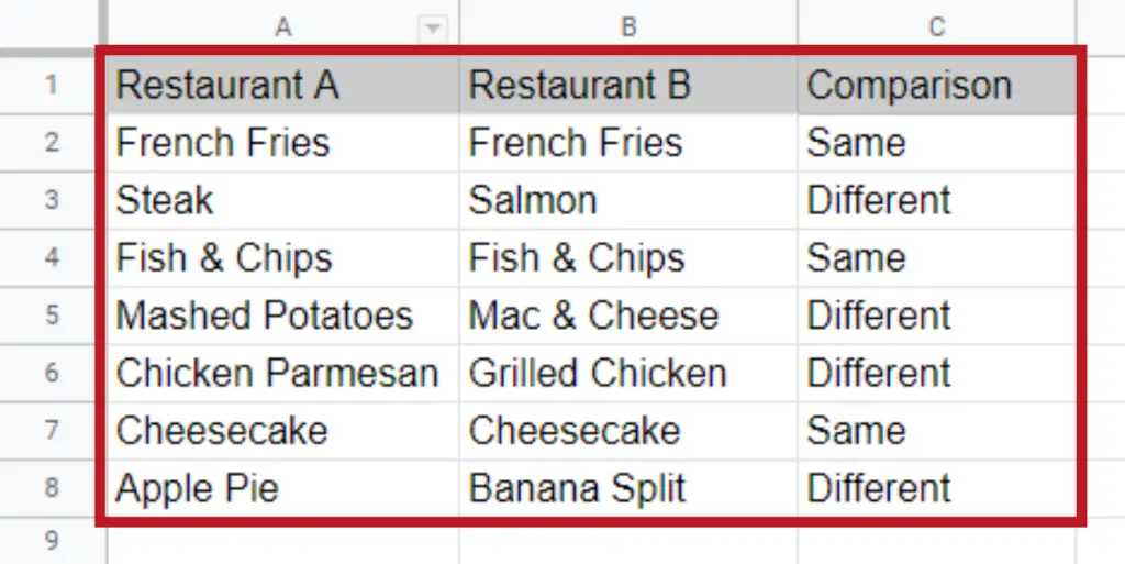
We’ll write a formula to compare two columns for a row that will give a predefined value in response. In this example we’ve defined ‘Same’ for similar/common entries and ‘Different’ for uncommon entries. Follow the below given steps:
Step 1 – Add an extra column
- Add an extra column in which the calculated comparison will be displayed.
- In this example, we named it ‘Comparison’
Step 2 – Enter the formula
- Select the top cell of the column. In our case, we are using ‘C2’.
- We will use the following formula Syntax=IF(Cell1=Cell2,”True Replacement Text”,”False Replacement Text”). In our case, we are comparing cells A2 and B2 and the replacement text for True is ‘Same’ and ‘Different’ for False text replacement. So, the formula will be:
=IF(A2=B2,”Same”,”Different”)
- Type the formula and press the ‘Enter’ button. You will get the result whether it’s Same or Different.
Step 3 – Apply the formula to whole column
- Now, drag the (■) symbol.
- Doing this will copy the formula to all the cells of the Comparison column.
Step 4 – Get the comparison of both menus

- The same menu items will be marked as ‘Same’.
- The uncommon/different items will be marked as ‘Different’.
These are just two of the several ways Google Sheets allows you to compare data across two columns. You can adapt these methods to make highly potent data comparisons depending on what you need Google Sheets to do. The applications can be as straightforward as organizing an inventory of your record collection or as intricate as examining a company’s product line.


