How To Color Code Drop Down List In Google Sheets

You can watch a video tutorial here.

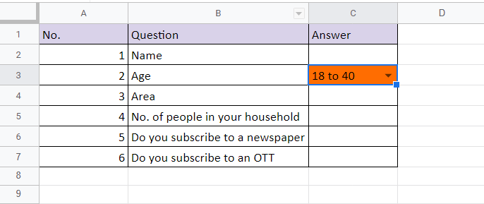
To validate the data that is entered in a cell in Google Sheets, it is possible to define the list of values that are allowed by creating a drop-down list. This is especially useful when creating data entry forms and you need to restrict the values that are entered. Having created a drop-down list you can then color code the values selected so that it is easier to differentiate the different responses.

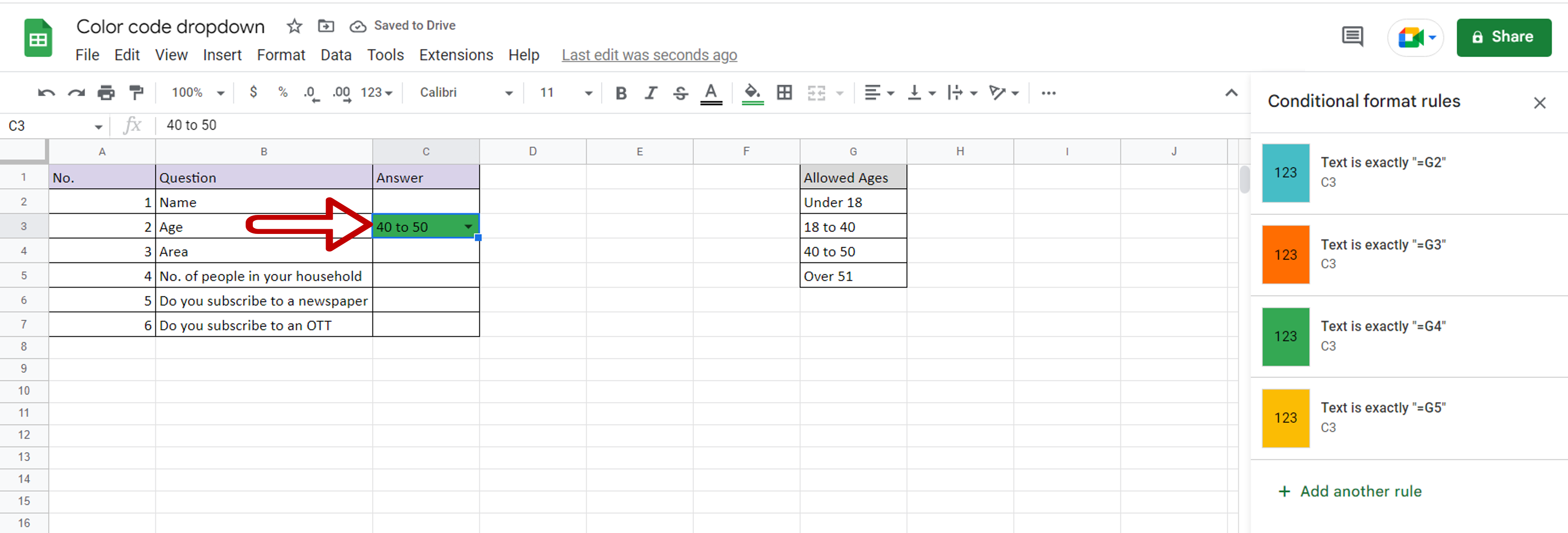
Step 1 – Open the Conditional format rules pane

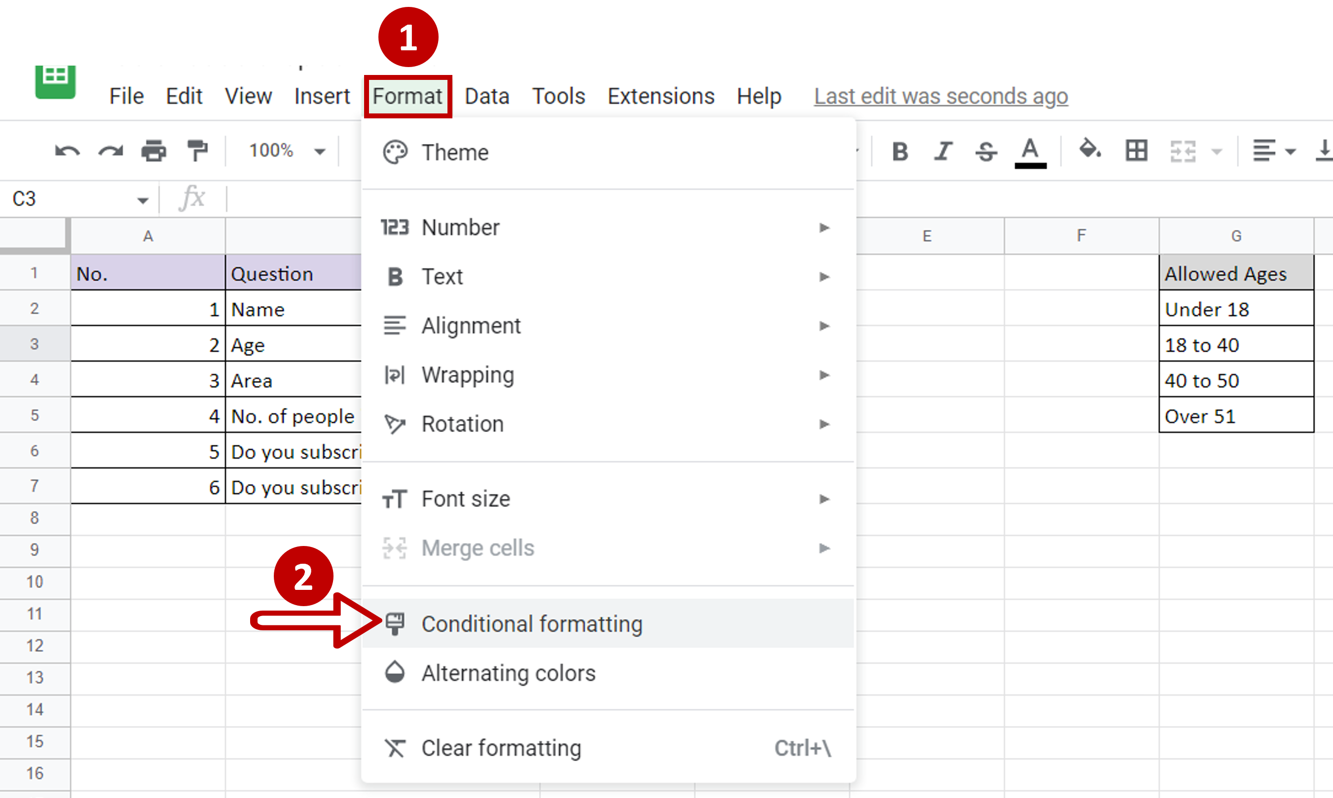
– Select the cell which contains the drop-down list
– Go to Format > Conditional Formatting

Step 2 – Create the rule for the first value

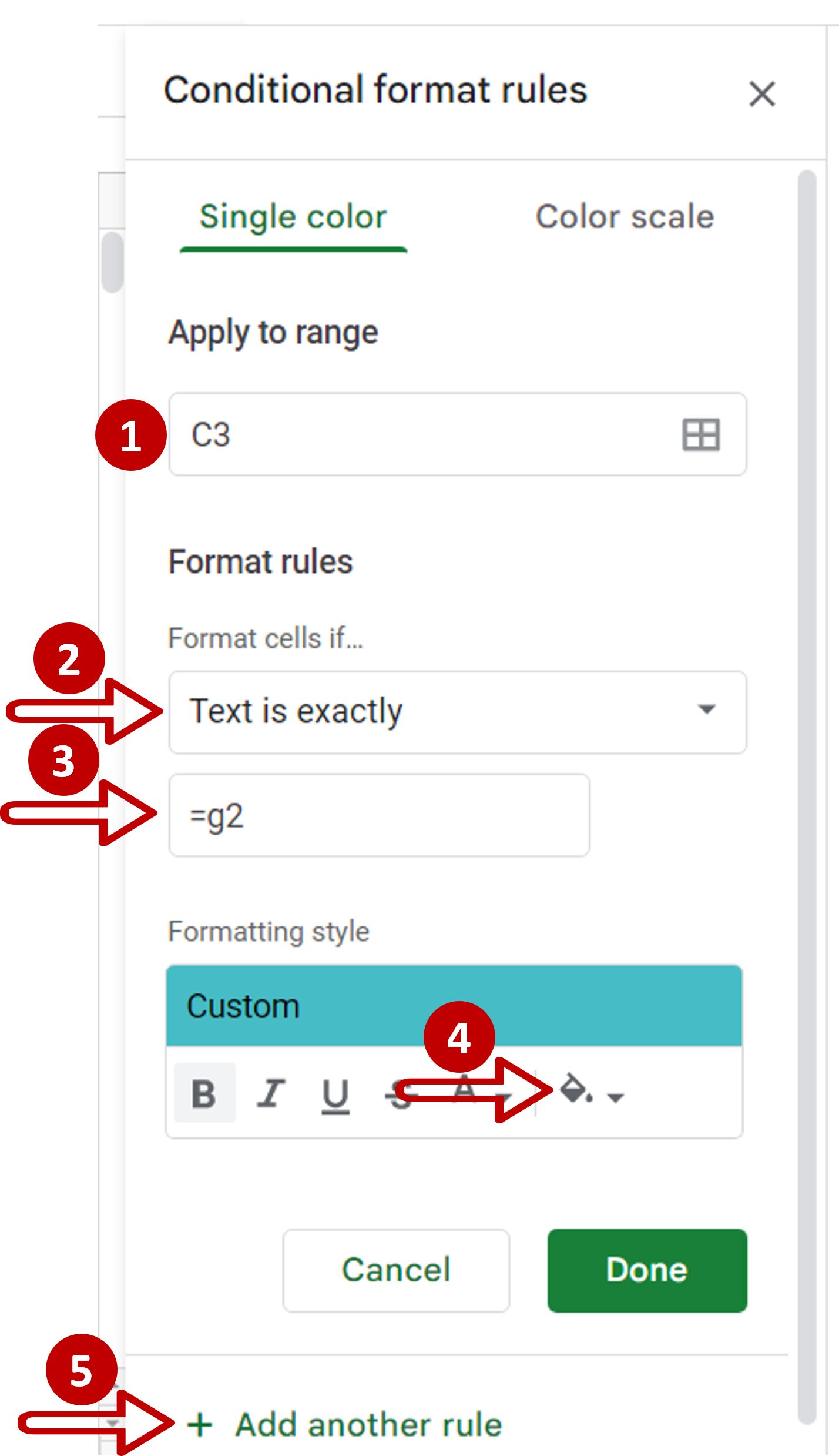
– Define the parameters:
>Apply to range: Leave ‘C3’
>Format cells if: Choose ‘Text is exactly’
Enter ‘=G2’
>Formatting style: Choose a fill color
– Click Add another rule

Step 3 – Create rules for the other values

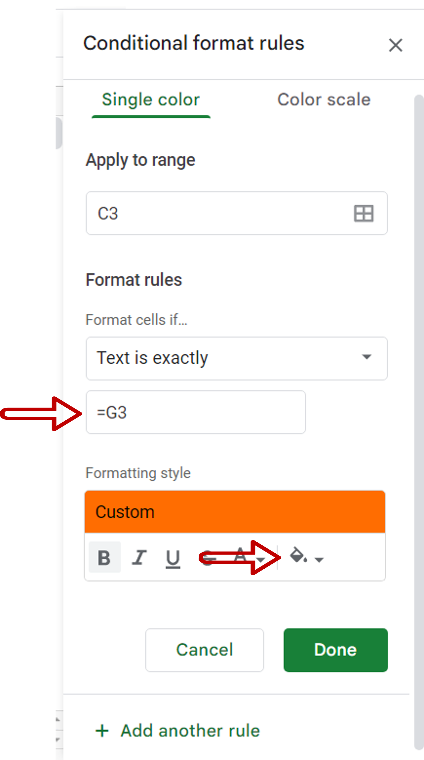
– Repeat Step 2 for the rest of the values in the drop-down
– Use the following cell references in each rule for the value under ‘Text is exactly’
>G3
>G4
>G5
– Change the color for each rule
– Click Done when all the rules have been added