
How to change the date format in Google Sheets
 By
SpreadCheaters
By
SpreadCheaters
Page last updated:
19/04/2023 |
Next review date:
19/04/2025
You can watch a video tutorial here.
In Google Sheets, you will frequently get to work with dates. Whether you are creating or editing a Google Sheet, you can format the date to be displayed in a style of your choosing. You can either choose one of the preset formats or define your own.
Option 1 – Use a preset format
Step 1 – Choose the date format
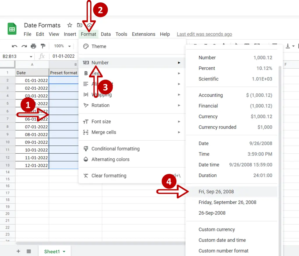
- Select the dates to be formatted
- Go to Format > Number
- Choose one of the preset date formats
Step 2 – Check the result
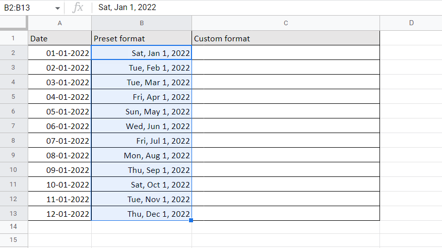
- Check that the date has been formatted correctly and increase the column width, if needed, by dragging the column divider
Option 2 – Create a custom format
Step 1 – Open the Custom date and time formats window
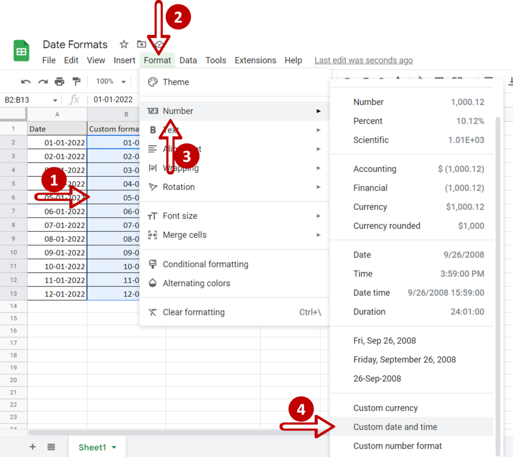
- Select the dates to be formatted
- Go to Format > Number
- Choose Custom date and time
Step 2 – Define the date format
- Change the format for the Month to the short name and delete the Day by placing the cursor after the hyphen following the Day and pressing Backspace on the keyboard twice (to delete the hyphen as well)
- Change the hyphen between Month and Year to a forward slash (/)
- Click Apply
Step 3 – Check the result
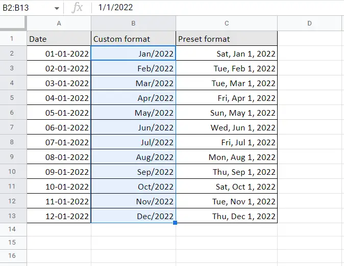
- Check that the date has been formatted correctly and increase the column width, if needed, by dragging the column divider


