
How do you lock cells in google sheets
 By
SpreadCheaters
By
SpreadCheaters
Google sheets offer a very interesting way to freeze panes. We can freeze single or multiple rows and columns in google sheets. We can perform the below mentioned way to use freeze panes to lock cells in google sheets:
We’ll learn about this methodology step by step.
Lock cells in google sheets:
Step-1: Google sheet with multiple columns and rows
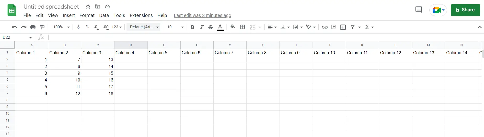
To do this yourself, please follow the steps described below;
– Open the desired Google Sheet which contains multiple columns and rows as we have in the image above
Step-2: Making the required cell active
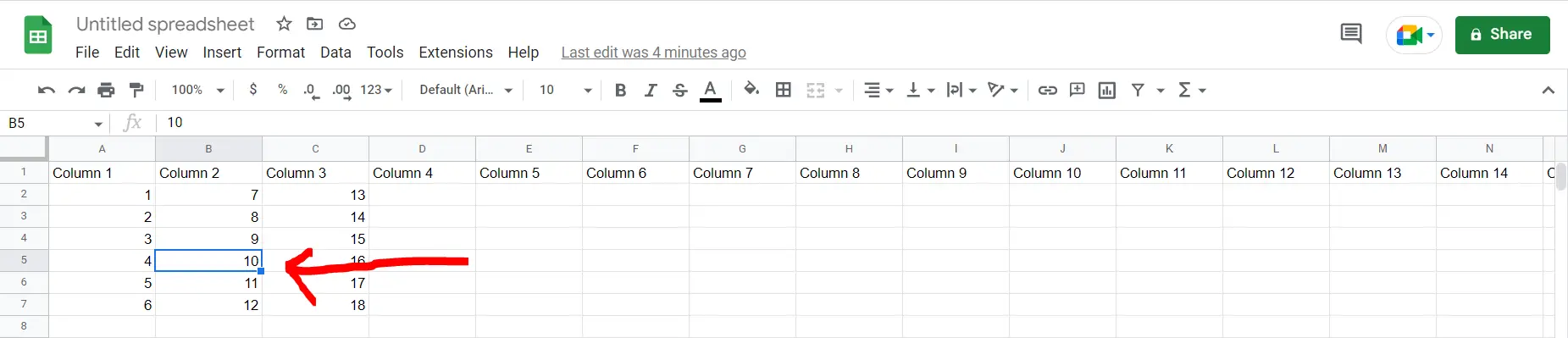
– Now select any of the required cells which need to be frozen.
Step-3 : Freezing the column
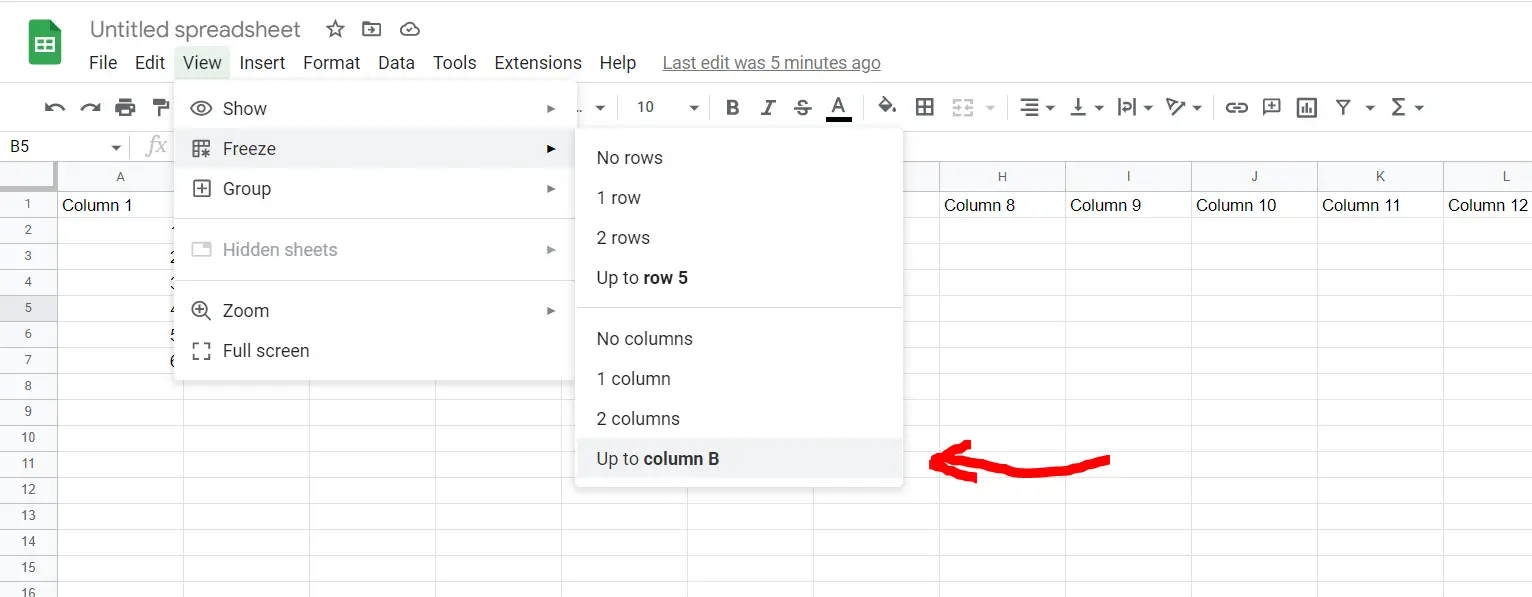
– Go to the View option, then click on “Freeze”, then click on “Up to column X”(Where X is the column of the active cell). This will freeze the column where we have our cell active (in our case column B)
Step-4 : Freezing the row
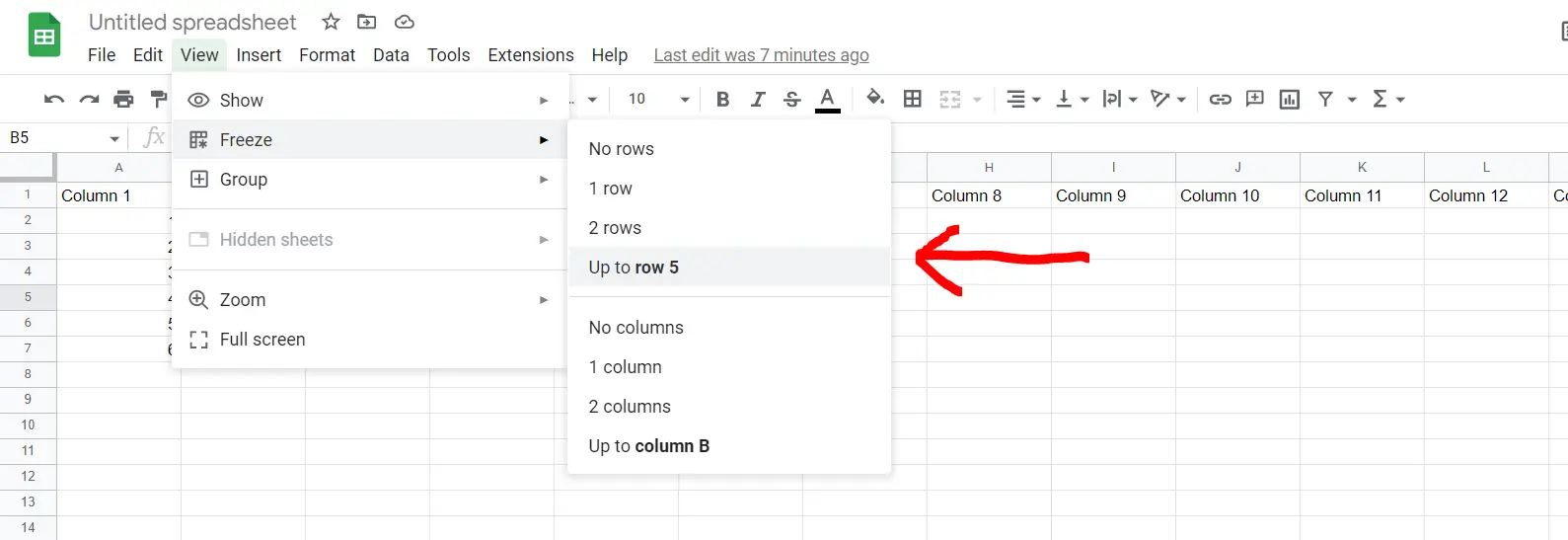
– Go to the View option, then click on “Freeze”, then click on “Up to row X”(Where X is the row of the active cell). This will freeze the row where we have our cell active (in our case row 5)
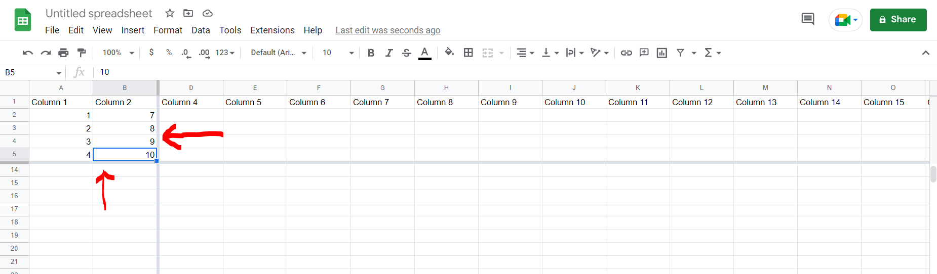
Final Image: Cell frozen
– We can now see that after scrolling towards the right or to the bottom, our selected cell remains stationary, hence we have locked the cell.


