
How do you freeze panes in google sheets
 By
SpreadCheaters
By
SpreadCheaters
Page last updated:
19/04/2023 |
Next review date:
19/04/2025
Google sheets offer a very interesting way to freeze panes. We can freeze single or multiple rows and columns in google sheets. We can perform the below mentioned way to freeze panes in google sheets:
- Freeze one column in Google sheets
- Freeze multiple rows in Google sheets
We’ll learn about this methodology step by step.
Option -1 Freeze one column in google sheets:
Option 1 (Step-1): Google sheet with multiple columns
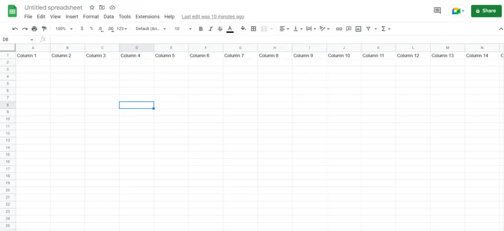
To do this yourself, please follow the steps described below;
- Open the desired Google Sheet which contains multiple columns as we have in the image above
Option 1 (Step-2): Making the required column active
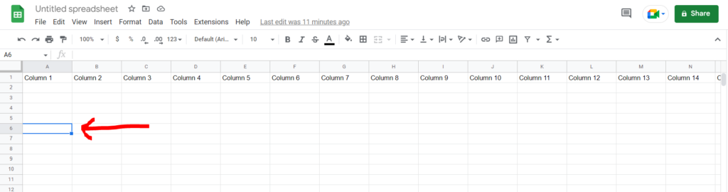
- Now select any of the required columns which need to be frozen.
Option 1 (Step-3) : Freezing the column
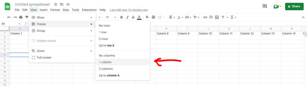
- Go to the View option, then click on “Freeze”, then click on “1 column”. This will freeze the column where we have our cell active (in our case column A)
Option 1 (Final Image) : Column has been frozen
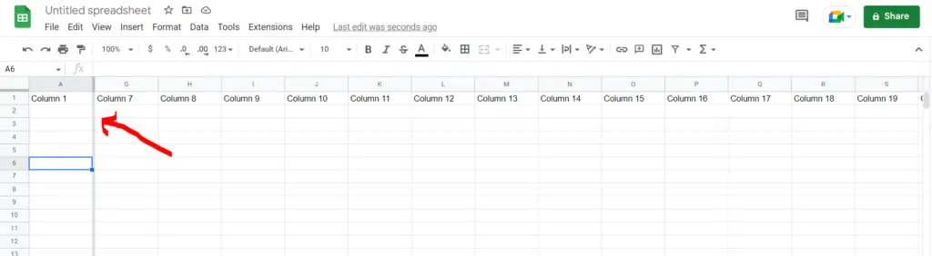
- Now after scrolling to the right, we can see that column A has been frozen.
Option -2 Freeze multiple rows in google sheets:
Option 2 (Step-1): Google sheet with multiple rows
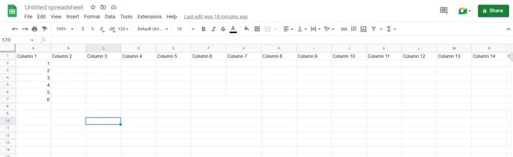
- Open the desired Google Sheet which contains multiple rows as we have in the image above
Option 2 (Step-2): Making the required row active
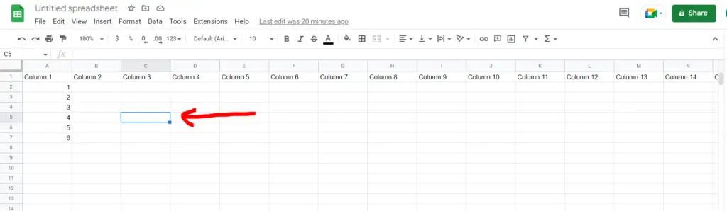
- Now select any cell in the required row which need to be frozen, along with all the rows to the left of it.
Option 2 (Step-3) : Freezing the row
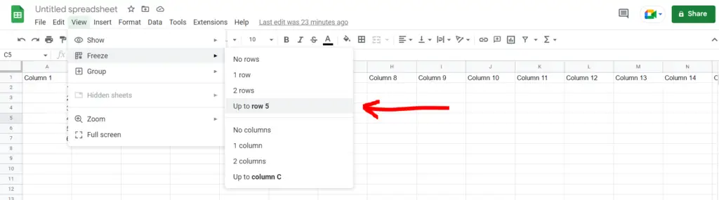
- Go to the View option, then click on “Freeze”, then click on “1 column” if you want to freeze the top row, or click on “Up to row 5” if you want to freeze all rows above the selected row and include it as well. This will freeze all the rows till the row where we have our cell active (in our case row 1-5)
Option 2 (Final Image) : Rows have been frozen
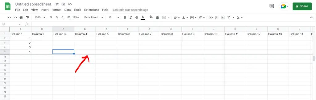
- Now after scrolling to the bottom, we can see that rows 1-5 have been frozen.


