
How do you freeze a column in google sheets
 By
SpreadCheaters
By
SpreadCheaters
Page last updated:
19/04/2023 |
Next review date:
19/04/2025
Google sheets offer a very interesting way to freeze a column. We can freeze single or multiple columns in google sheets. We can perform the below mentioned way to freeze a column in google sheets:
We’ll learn about this methodology step by step.
Freeze a column in google sheets:
Step-1: Google sheet with multiple columns
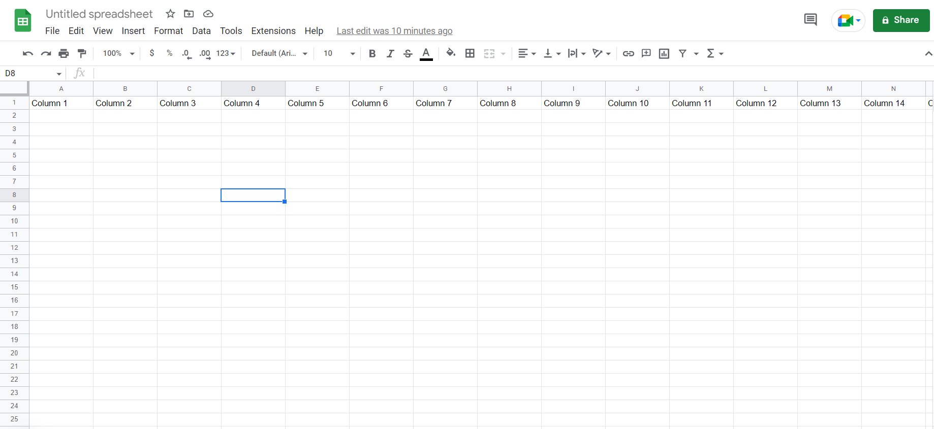
To do this yourself, please follow the steps described below;
– Open the desired Google Sheet which contains multiple columns as we have in the image above.
Step-2: Making the required column active
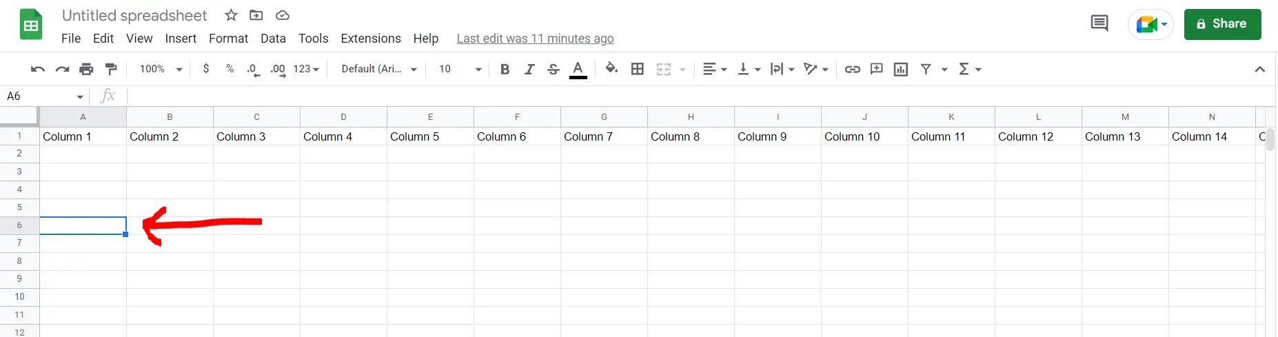
– Now select any of the required columns which need to be frozen.
Step-3 : Freezing the column
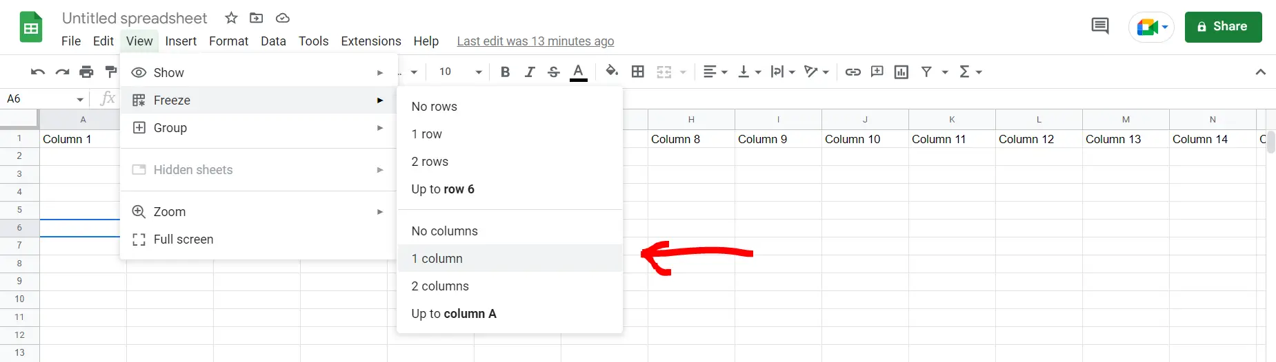
– Go to the View option, then click on “Freeze”, then click on “1 column”. This will freeze the column where we have our cell active (in our case column A)
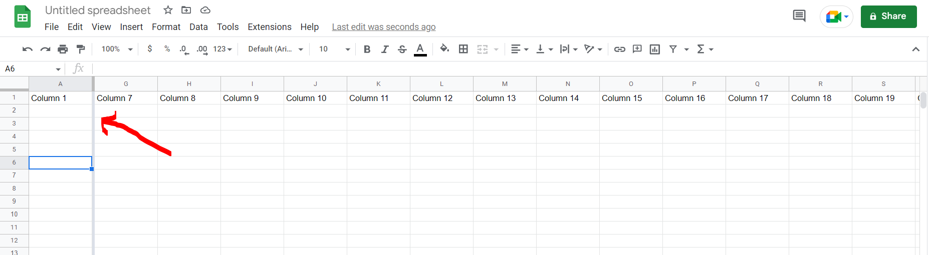
Final Image : Column has been frozen
– Now after scrolling to the right, we can see that column A has been frozen.


