
How to freeze multiple rows in Google Sheets
 By
SpreadCheaters
By
SpreadCheaters
Page last updated:
19/04/2023 |
Next review date:
19/04/2025
You can watch a video tutorial here.
Freezing is commonly used when scrolling through large amounts of data on a worksheet. You can freeze multiple rows either to compare rows in distant sections of the worksheet or to keep header rows in place while scrolling down.
Step 1 – Navigate to the Freeze menu
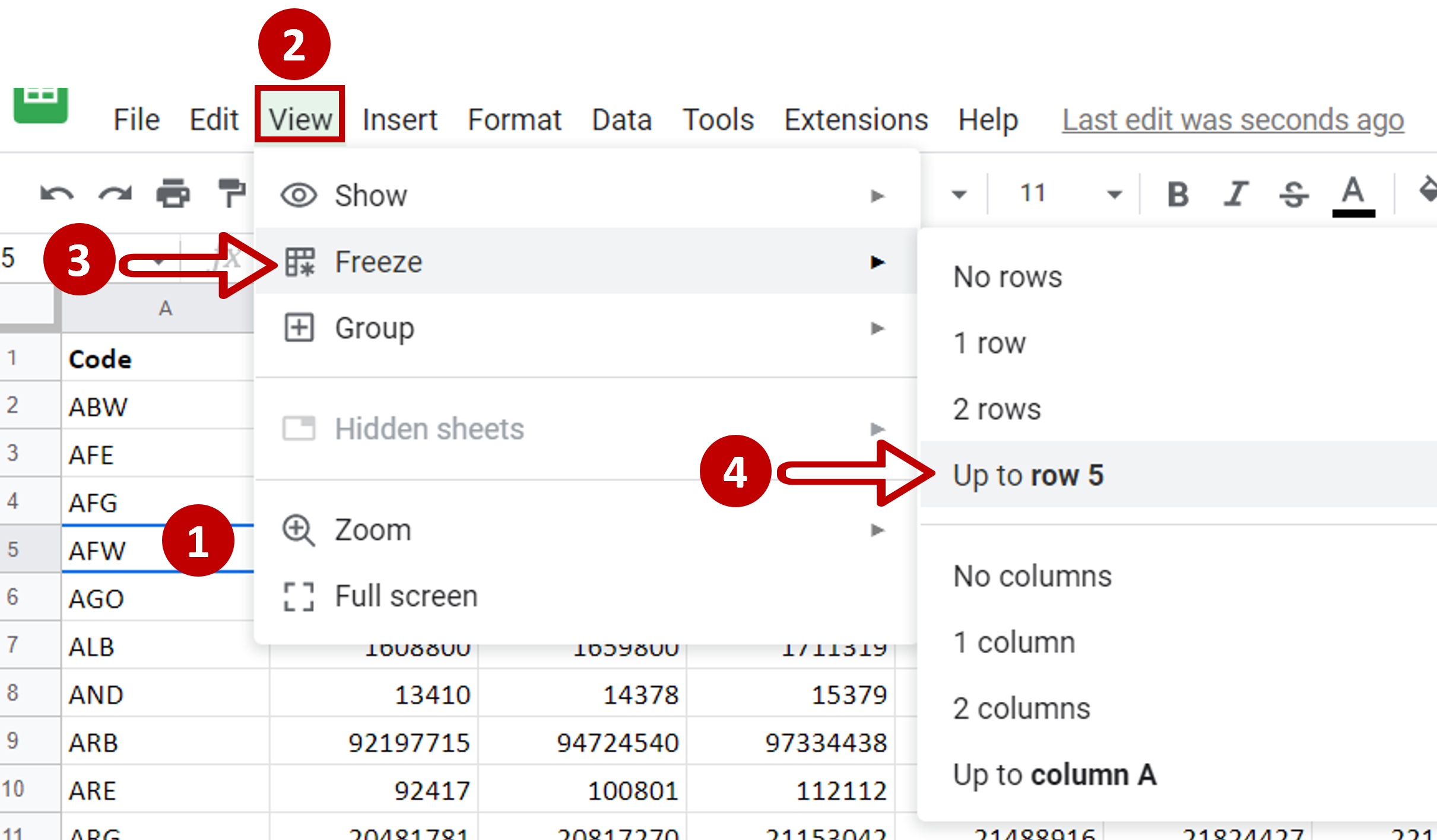
– Place the cursor in the row up to which the rows are to be locked
– Go to View > Freeze
– Select Up to row 5
Step 2 – Check the result
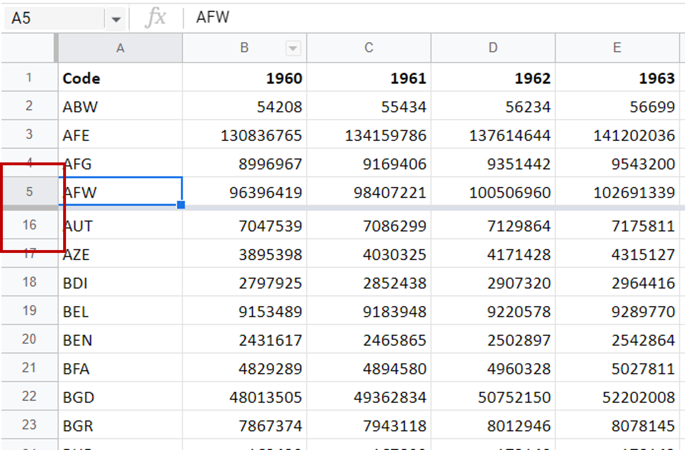
– Scroll down to check that the column header stays in place


