
How to create a scenario pivot table in Excel
 By
SpreadCheaters
By
SpreadCheaters
Our dataset contains information about a store’s financial performance over 5 years, including its income, expenses, and profits. We want to create a scenario pivot table that will allow us to analyze how changes in income and expenses will affect the store’s profits. To do this, we will use the Scenario Manager feature.
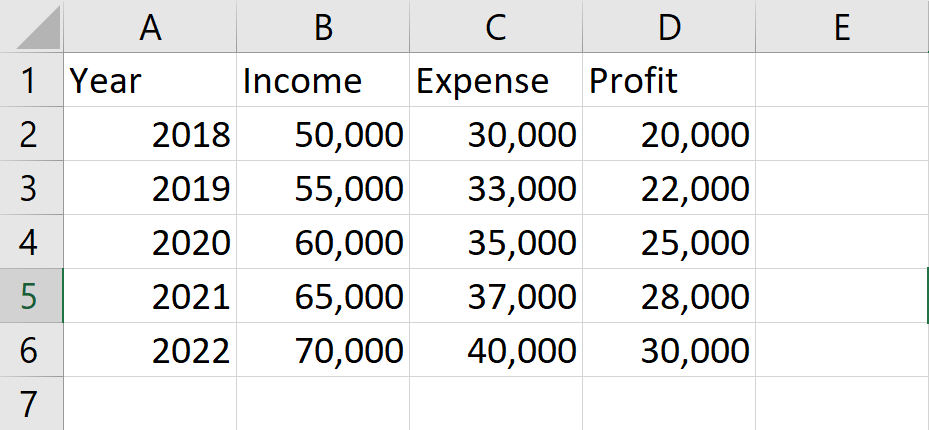

Creating a scenario pivot table in Excel involves using different assumptions or scenarios to analyze how they impact a particular outcome or result. In the case of financial analysis, scenarios can include best-case, worst-case, and expected-case scenarios that are used to understand how changes in various factors like revenue, expenses, or market conditions can impact the financial performance of a business.
Step 1 – Click on the What If Analysis option
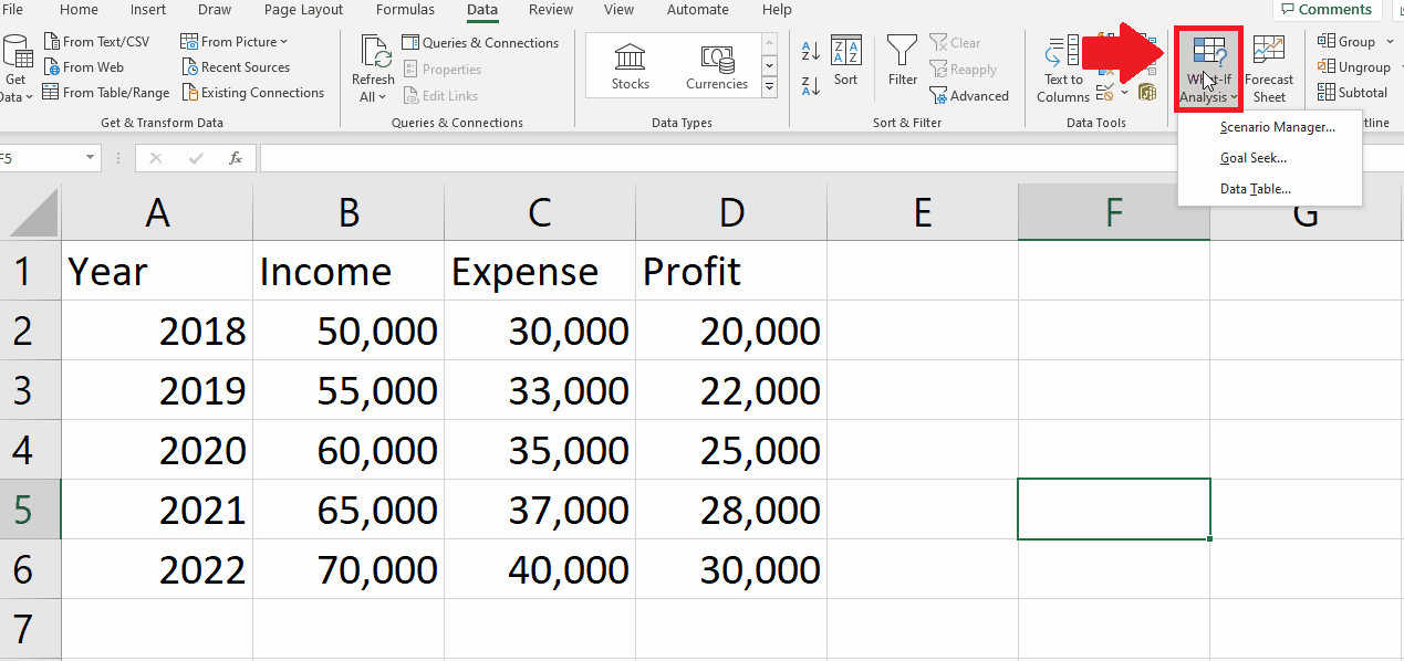
– Right Click on the What If Analysis option in the Forecast group of the Data tab and a drop-down menu will appear
Step 2 – Click on the Scenario Manager option
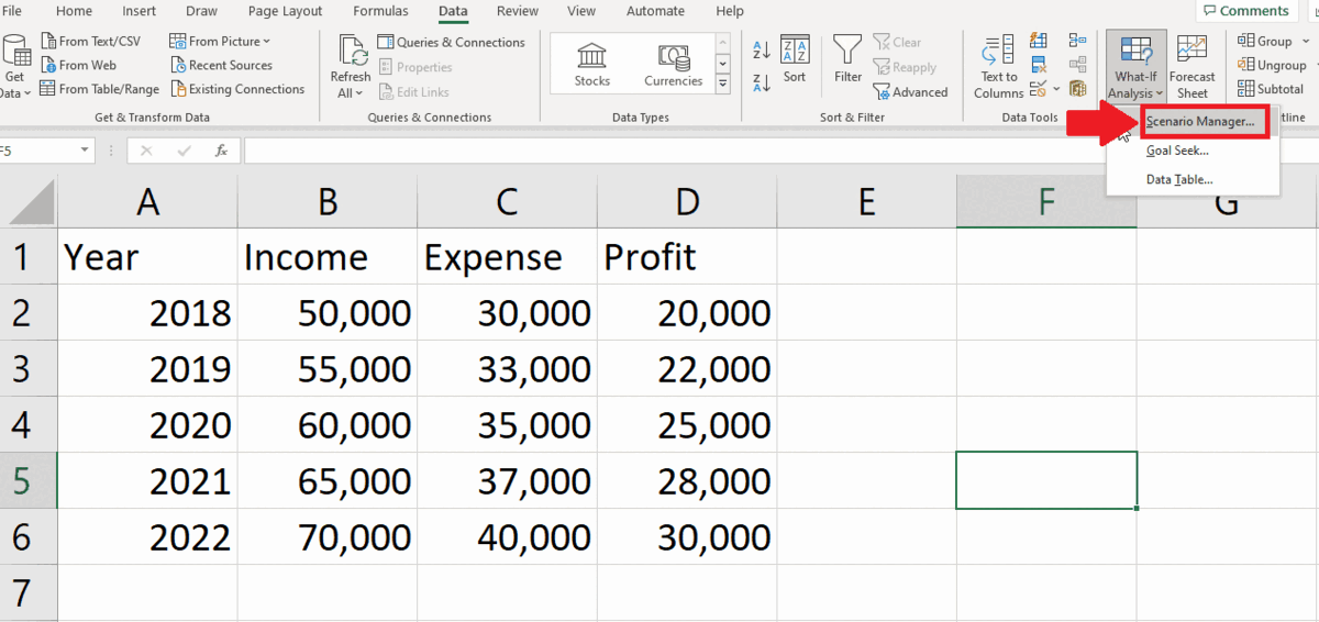
– From the drop-down menu, click on the Scenario Manager option and a Scenario Manager dialog box will appear
Step 3 – Click on the Add option
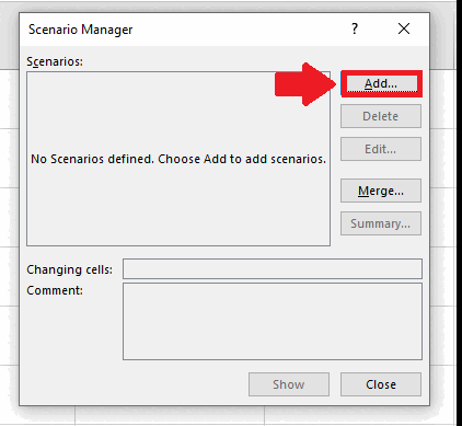
– From the dialog box, click on the Add option and a Add scenario dialog box will appear
Step 4 – Select the Name of the Scenario
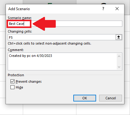
– Type the Scenario option in the box below the Scenario Name option
– Here we have selected “Best Case” as a name. You may select any other name
Step 5 – Select the Changing cells
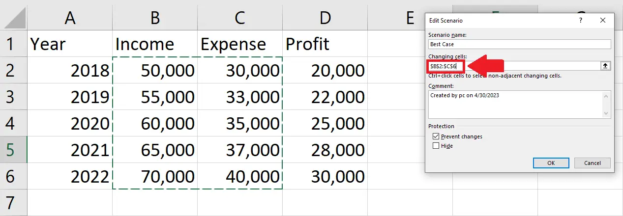
– After selecting the name, select the range of cells that you will change
– Here we have B2:C6
Step 6 – Click on OK
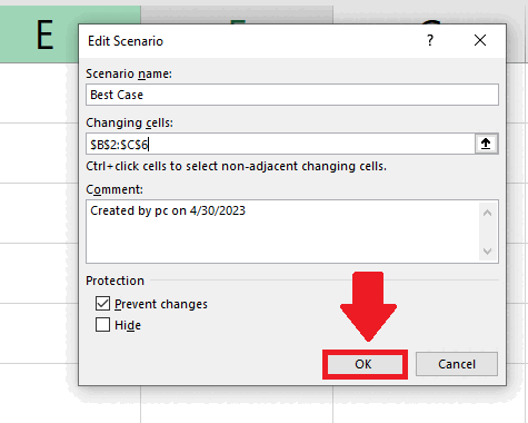
– After selecting the range of changing values, click on Ok and a Scenario values dialog box will appear
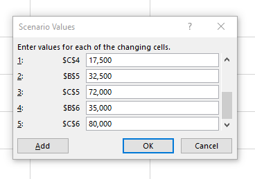
Step 7 – Change the values
– In the Scenario Values dialog box, change the values as you want
– Here we have doubled the Income and half the Expense
– You may select any other scenario based on your requirements
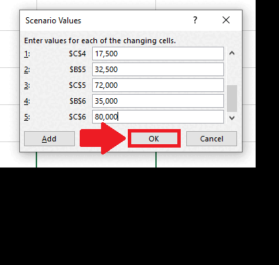
Step 8 – Click on OK
– After changing the values, click on OK and Scenario Manager dialog box will appear
Step 9 – Click on the Add option
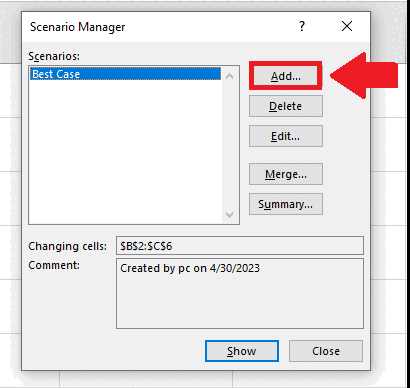
– From the dialog box, click on the Add option and a Add scenario dialog box will appear
Step 10 – Select the Name of the Scenario
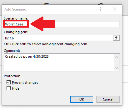
– Type the Scenario option in the box below the Scenario Name option
– Here we have selected “Worst Scenario” as a name. You may select any other name
Step 11 – Select the Changing cells
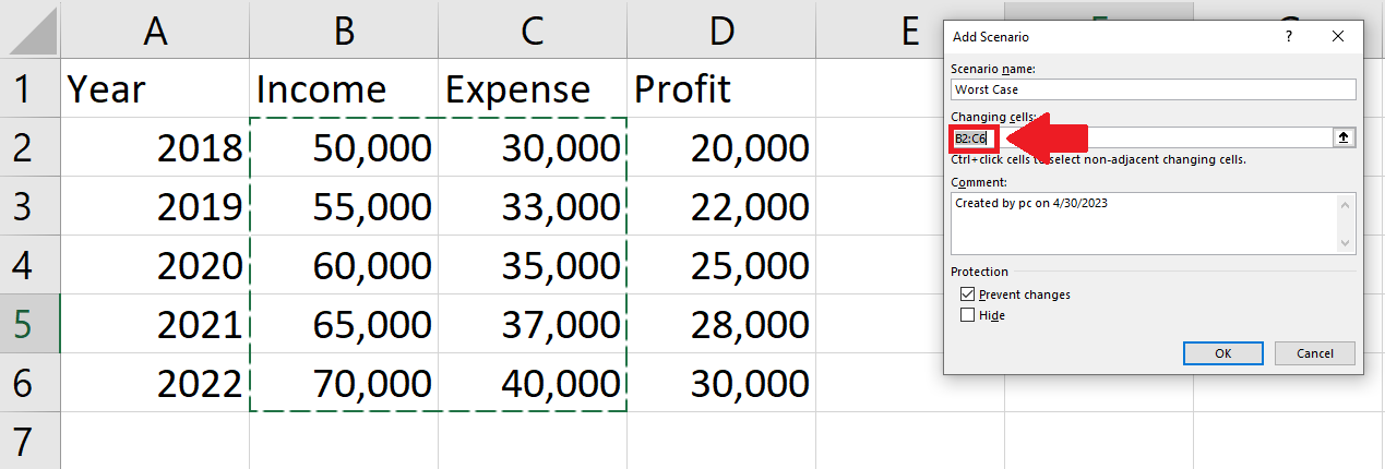
– After selecting the name, select the range of cells that you will change
– Here we have B2:C6
Step 12 – Click on OK
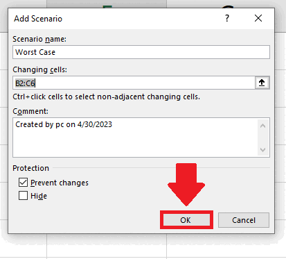
– After selecting the range of changing values, click on Ok and a Scenario values dialog box will appear
Step 13 – Change the values
– In the Scenario Values dialog box, change the values as you want
– Here we have doubled the Income and half the Expense
– You may select any other value
Step 14 – Click on OK
– After changing the values, click on OK and a Scenario Manager dialog box will appear
Step 15 – Click on the Summary option
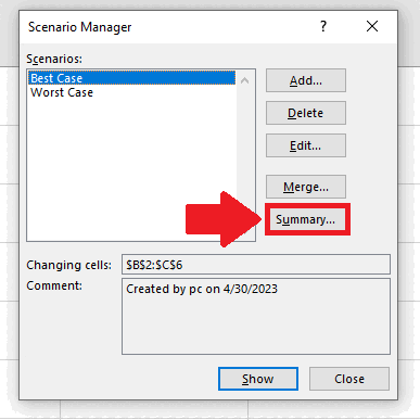
– In the Scenario Manager dialog box, click on the Summary option and a Summary dialog box will appear
Step 16 – Click on the Scenario Pivot report option
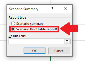
– In the Scenario Summary dialog box, tick the checkbox of the Scenario Pivot report option
Step 17 – Select the Result cells
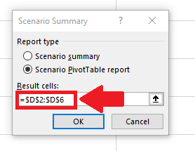
– After clicking on the check box, select the range of cells that you want to change by changing the values selected at the start(income, expense)
– Here we selected D2:D6 as the range of cells that will automatically change after changing values in scenarios
Step 18 – Click on OK

– After selecting the result range, click on OK to get the required result


